Improving Seismic Data Quality by Reprocessing and Redesign of a 3D Survey in an Area of Chaotically-scattered Source-generated Noise

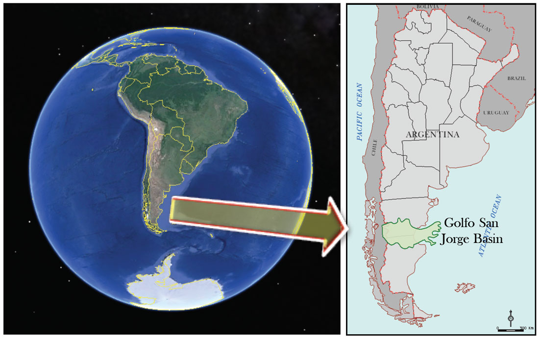
The purpose of this paper is to propose a two-fold solution to a complex noise problem in the Gulf of San Jorge Basin in Argentina. Irregularly shaped intrusive bodies scattered at shallow depths over large areas above the reservoir generate a severe signalto- noise problem that masks deeper reflection signals and inhibits the ability to find prospects. This type of noise is source generated and scatters in a chaotic manner. In order to tackle this problem, a custom tailored present-day reprocessing flow is applied to enhance the data quality below the intrusive areas. Significant improvement is observed with regards to reflection continuity, character and frequency content. Nevertheless, the data improvements are not sufficient for reliable interpretation of reflection amplitude and character and a new 3D survey design is proposed. The 3D design focuses on proper sampling of the noise to improve signal to noise ratio, type and magnitude of noise present, as well as on signal. Two models using different sets of acquisition parameters are proposed, the alternate and recommended, and then compared to those used in the original acquisition. The new sets of parameters have a higher trace density produced by the reduction of line spacing and have a significant impact on costs. It is important to visualize what the potential benefit may be. A special tool called Data Simulation is applied using local super gathers and the geometry of each survey to simulate stacked sections. In this studied case, it appears that increased design density may be expected to provide the increase in data quality desired by the interpreter in the poor data areas. Data Simulation helps decrease the uncertainty in acquisition parameter selection. Both solutions worked well and required the interaction of many professionals in the processing and the design stages.

Introduction

In the Cretaceous section in the Gulf of San Jorge Basin, Argentina, the Pozo D-129 formation is considered the primary source rock. Production comes from the inter-bedded fluvial and lacustrine sandstones of the Mina del Carmen and Comodoro Rivadavia formations. In the 3D seismic study area, the Pozo D-129 formation lies between 1700 m (below sea level) in the northern part of the study area to 2200 m in the southern part. The Comodoro Rivadavia “K” level lies between 600 to 900 meters below sea level and the “M7” level lies between -900 to -1200 meters below sea level (Figure 1). This information will be used in both the processing and design stages.

In the stratigraphic column of the basin there are intrusive bodies, sometimes of considerable areal extent and of varied geometries. These bodies manifest at shallow levels in general and sometimes are parallel with the stratification and other times, they cut several meters of the geological column acquiring diverse geometric forms linked to the mechanism of the intrusion.

These bodies appear as many lenses of irregular shapes whose edges act as energy diffraction points. These diffractions interact in a chaotic manner. The thickness of the intrusive bodies is considerable (tens of meters in some cases), so they reflect a large amount of seismic energy at the time of recording. This results in reflection signals with very low amplitudes that get masked in the presence of high amplitude scattered noise (Figure 2a and 2b).

In some areas of the basin, these bodies are located above the production zones or in prospective areas, which means that the lack of reliable information below them creates situations of uncertainty in the continuity of the reflectors and in the geometry of possible traps in the areas of interest.

It is necessary to look for a strategy that allows the improvement of the information below these true masking screens to the seismic data.

A partial solution comes from data processing, which has shown by designing a processing flow specific to the problem that a considerable improvement in the quality of the information is achieved. Where this is not a sufficient option for the complexity of the situation, then the alternative of a methodology of 3D seismic design is presented. It addresses the challenge of obtaining new data that better samples the source-generated noise, and results in improved seismic information.

To accomplish this last objective one has to have in mind that the design of 3D seismic programs must anticipate the surface sampling requirements necessary to properly record elements of the emerging wavefield that are relevant to desired target reflectors. However, parameters that are sufficient to measure desired reflection signals should not be the only consideration. In many areas, it is also important to consider the type and magnitude of noise. In particular, areas with a strong occurrence of chaotically-scattered, source-generated noise require special attention.

In the study area, a 3D seismic project was recorded in 1997 and has been used to demonstrate the application of a design method for a new acquisition. Now, this seismic is being reprocessed up to Prestack Depth Migration (PSDM), to obtain the best possible data. The original design did not take into account the presence of igneous bodies because they were not detected with the previous 2D lines.

Finally, the seismic interpretation performed on the new information will lead to the identification of new areas for drilling, which were previously masked by the poor quality of the available data. This information treatment will certainly enable attribute analysis and special seismic processes to optimize future prospects.

Improving quality through specific data reprocessing

The work plan was to design a processing flow interacting systematically with the seismic interpreter. This allowed specific focus on the problem of the shadow in the seismic data in order to improve its quality, transform it into reliable data for interpretation and of course, to minimize data deterioration in the rest of the zone. To achieve this objective, it was very important to integrate the interdisciplinary work group composed of Geophysicists, Geologists and Reservoir Engineers and the proactive communication amongst them.

Having clarified the proposed objective and the scope of the problem, then as a first step, the field data was loaded and reformatted, the geometry building, positioning of lines and bins was done, and a Minimum Phase Filtering was performed. A synthetic sweep was created using the original sweep parameters (i.e. frequency range, sweep length, tapers, etc.), a zero-phase wavelet was extracted from the autocorrelation of the sweep and a Minimum Phase Filter was derived from the extracted wavelet and convolved with the input data. This converts the correlated data to minimum phase.

In order to attenuate the noise in the shot domain a proprietary noise attenuation workflow was applied to each shot. The workflow consists of analyzing different frequency bands and identifying the high amplitude noise and the signal, followed by an adaptive filter that puts together the signal with the attenuated noise. The root-mean-squared (RMS) amplitude is calculated to put a threshold for what should be noise and signal.

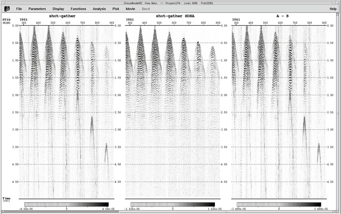
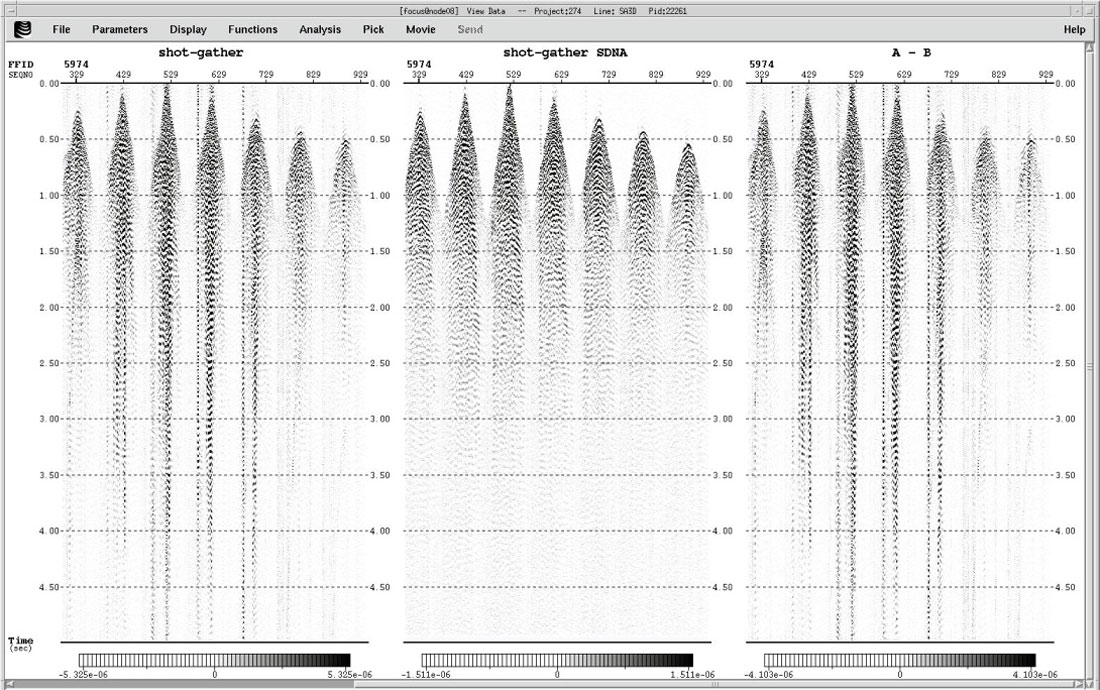
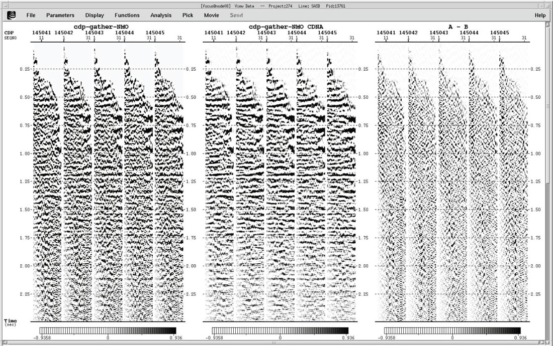
In this dataset, nine frequency bands were selected as follows: 0-5, 5-10, 10-15, 15-20, 20-30, 30-40, 40-50, 50-60 and 60-125 Hz. After applying the workflow, the difference between the input and the output was calculated to ensure that no coherent signal was attenuated. The resultant data was also stacked to ensure the improvement in the image. Results of the noise attenuation can be seen in Figure 3 for the shot domain noise attenuation and Figure 4 for the CDP domain noise attenuation.

For static corrections calculation, the delay time method used GLI (Generalized Linear Inversion).

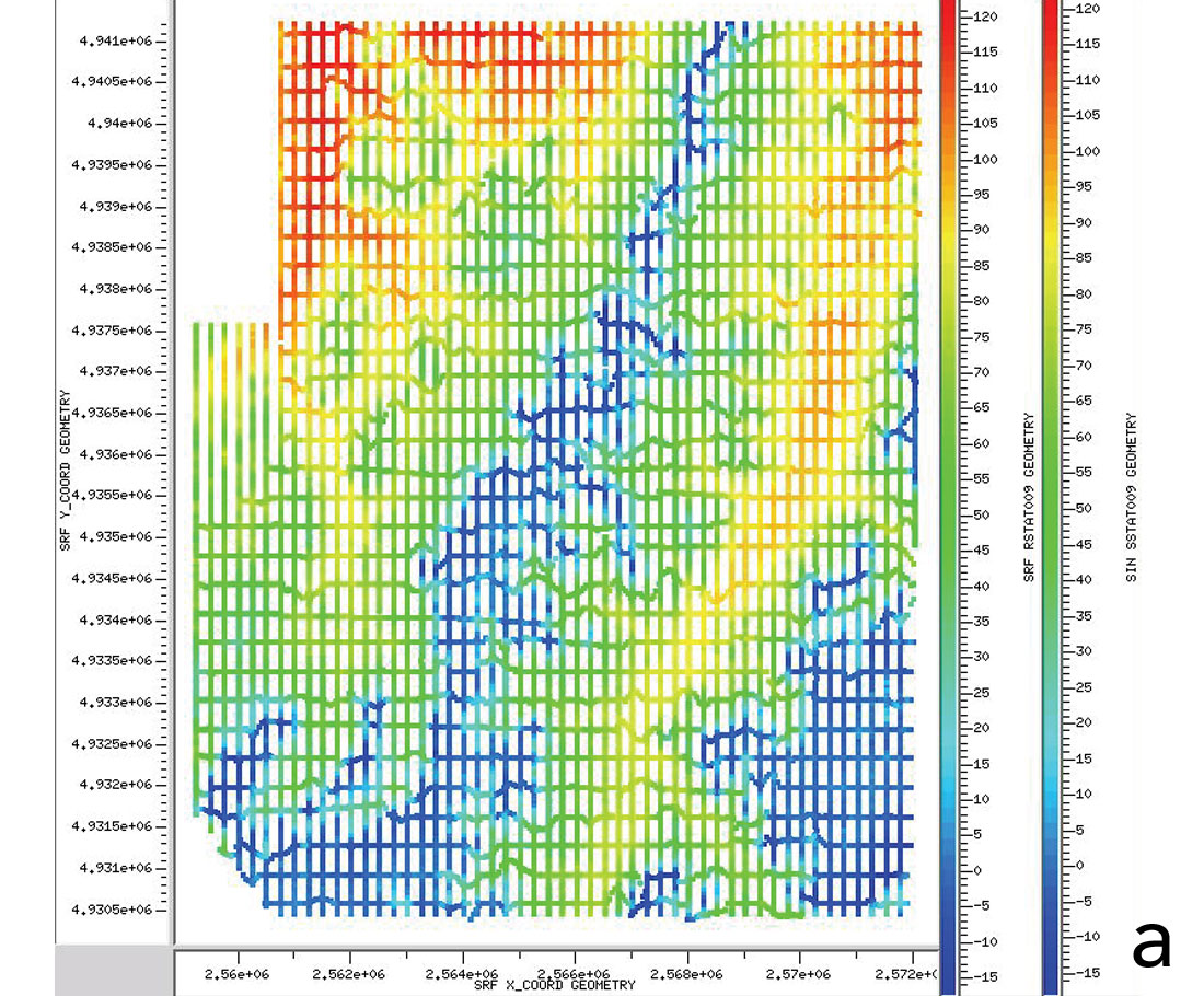
A one-layer weathering model was chosen. The offset for refractor velocity calculation was 200-2500 m. A constant weathering velocity of 1000 m/s was used. The refractor velocity was 2000-3000 m/s and the replacement velocity was 2000 m/s. The final results of the refraction statics can be observed in Figure 5a).

In order to determine the best parameters to correct for spherical divergence and Inelastic Attenuation, detailed tests were performed.

After analyzing those results it was decided to use a Time-Power curve with an exponential factor of 1 from 0 to 1250 ms and a constant from 1250 ms onwards.

It was very important at this step to consider surface consistent amplitude compensation. Once these corrections were applied, we calculated surface consistent amplitudes using receivers, shots, and offsets. A noise reduction by Air Blast Attenuation (ABA) was also applied before the analysis.

Then, using the amplitudes’ mean values, we performed a trace rejection with “out of range” amplitudes. At this point it was important to analyze the amplitudes in order to eliminate just the anomalous ones and to keep balanced the amplitudes between the different surveys.

Finally, with the compensated amplitudes, a deconvolution (see next point for description) and a new Air Blast Attenuation (ABA) were applied. After deconvolution final surface consistent amplitude compensation was applied.

For the surface consistent deconvolution an initial autocorrelation and power spectrum were run. Deconvolution parameters were tested and the results were: surface consistent predictive deconvolution with an operator length of 160 ms, prediction distance of 16 ms, white noise 0.1 % on source, receiver and offset components.

The velocity analyses were performed using Semblance, Gathers, Dynamic Stack and Constant Velocity Stack (CVS). There was one velocity analysis every square kilometer before first residual static calculation, and four every square kilometer after the second residual static calculation. This step was one of the more time consuming and required more dedication to see some information in the conflictive data continuity sections.

After the first velocity analysis, an Iteratively Re-weighted Least Squares (IRLS) optimization was performed for residual statics calculation.

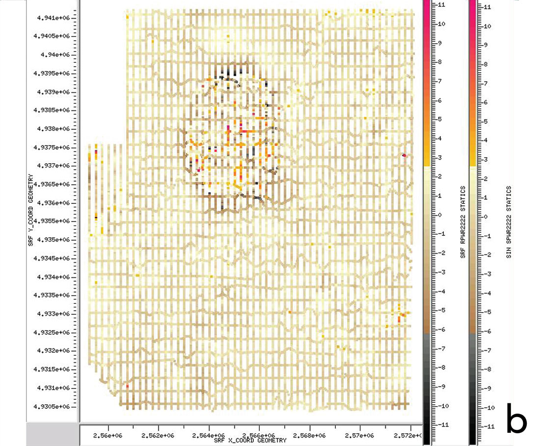
These static corrections are surface consistent with an analysis window width of 400 ms to 2000 ms. After the second Velocity Analysis, a second pass of IRLS was run with the same parameters to diminish dispersion. The results are displayed in Figure 5b).

Trim statics were applied with a maximum shift of 8 ms, a correlation window of 100-2000 ms and time-varying trims with a window length of 200 ms.

In order to attenuate the noise in the CDP domain a proprietary noise attenuation workflow was applied to each shot.

The workflow is similar to the SDNA (Shot domain Noise Attenuation) and consists in analyzing different frequency bands and identifying the high amplitude noise and the signal, followed by an adaptive filter that puts together the signal with the attenuated noise. The RMS amplitude is calculated to put a threshold for what should be noise and signal (as mentioned before, nine frequency bands were selected) (Choo et al., 2003).

To obtain a homogenous distribution of offsets and compensate for the low fold areas, a pre-stack 5D Regularization and Interpolation workflow was applied (Xu et al., 2010 and Liu and Sacchi, 2004).

The 5D Regularization and Interpolation methodology incorporates 5 dimensions (Time, IL, XL, Offset, and Azimuth). We incorporate variable azimuth spacing as a function of offset, where the larger offsets have larger sampling of azimuths. The 5D Spiral Regularization and Interpolation Parameters were: Offset Bins: 1-54 (50-2700, every 50), Patch size: 30x54x40x40 (azimbin, offbin, IL, XL), Method: Matching Pursuit, Max Dip: 10 ms/trace, Max K: 0.25 – 0.5 – 0.5 – 0.5 (azimbin, offbin, IL, XL).

This procedure results in a surface and sub-surface consistent regularization and interpolation that helps in the migration process and compensates acquisition gaps, while also accounting for azimuthal variations in the data.

Aperture tests on several target lines were performed to define a migration aperture in the x-t domain, considering the offsets to be migrated. After reviewing the test a 30 degree angle was chosen. A 3D Kirchhoff Pre-Stack Time Migration (PSTM) was run on the volume and new semblances (four velocity analyses every square kilometer) were created to do the residual velocity analysis. Finally, another PSTM with the refined velocity was performed (Migration Aperture of 30 degree maximum angle and offset distribution 50-2700m every 50 m).

In the post processing step, the following post-stack processing were tested and applied: FXY Decon, Dip Scan Stack, Time-Varying Bandpass filter, and AGC (500 ms).

We made a second version of the PSTM gathers using prestack spectral balancing to enhance frequencies.

As said before, the main objective of this project was to get better seismic information below some geological events such as basalt intrusive bodies. The data was acquired using vibroseis as the energy source, with the limitations of that time. Since this was a structural Oriented Processing, special care was taken with velocities, interpolation and migration (Figure 6a and 6b).

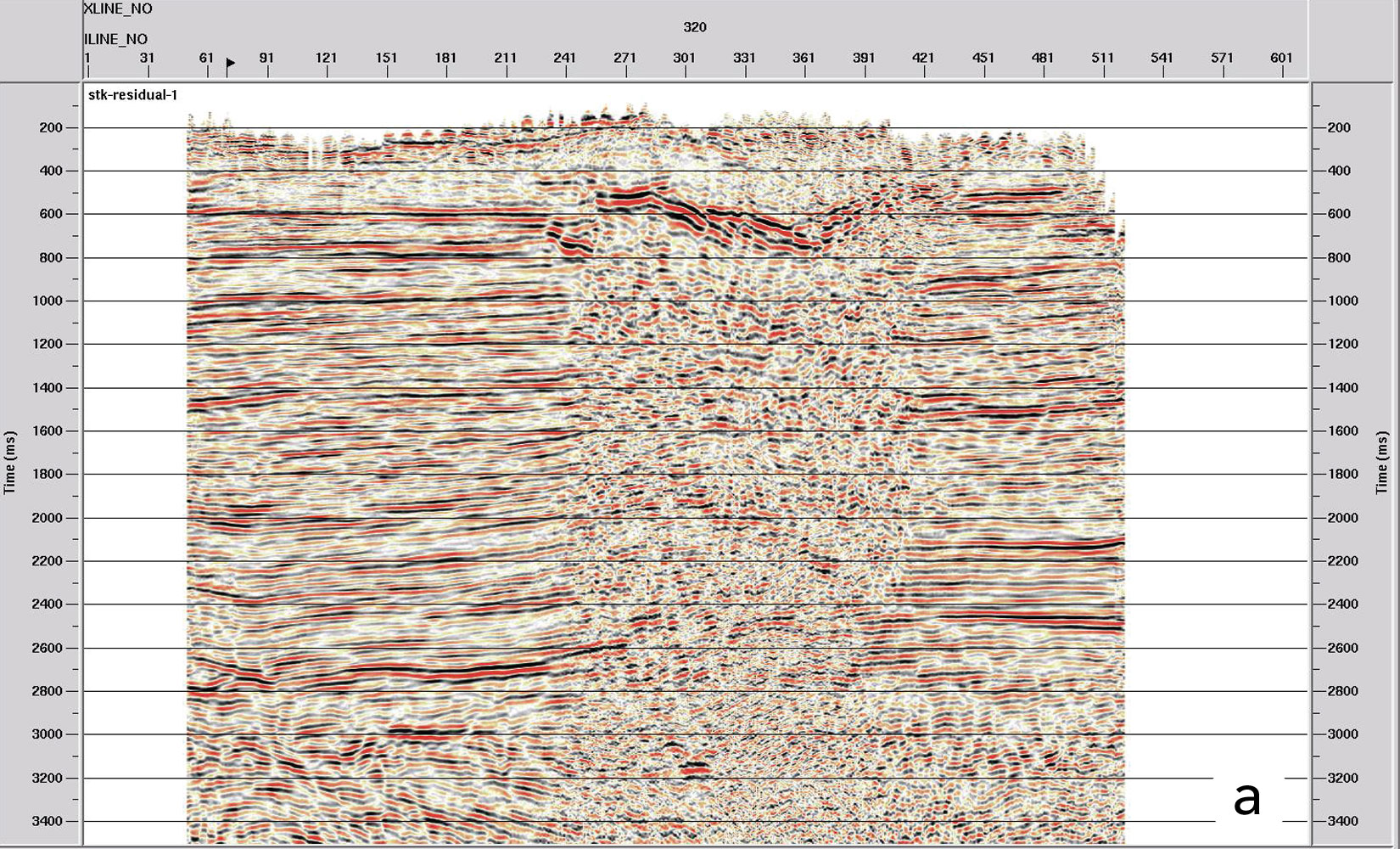
This treatment of the seismic data has been applied in the study area and remarkable results have been achieved regarding the quality obtained (Figure 7a and 7b). Results related to reflector continuity, frequency content and seismic character of the events are visible, which will have a favorable impact on the workflow of the seismic interpretation.

Optimizing 3D Design

Although this data processing flow yielded an important improvement in the data quality, in many cases the level of quality reached is not enough to solve certain structural schemes and stratigraphic configurations. These cannot be solved due to the deterioration of the signal to noise ratio associated with the mentioned volcanic events.

This situation must be solved by designing a new seismic survey. The survey must provide better sampling of both signal and noise so the interpreter may have better quality information. The study area and available background have been taken into consideration in the 3D design proposal examined next.

The 3D study area was designed and recorded in 1997 using I/O System Two recording equipment with Litton RHV 321 60.000 lb vibrators and Pelton Advance II control system. Source and receiver intervals (Si, Ri) were both 50 meters, receiver line spacing (RL) was 250 meters and source line spacing (SL) was 350 meters. This conventional design for this area leads to parameters that are sufficient to produce good data where noise due to the volcanic lenses is not present.

Applying standard 3D design formulae, it was confirmed that the receiver and source intervals, receiver and source line spacing used during the 1997 acquisition were appropriate for a 22 fold survey at the “M7” target levels (using offsets 0-1.670 m). Nevertheless, the patch used (10 x 98) is somewhat narrow compared to the desired cross-line aperture. This may be justified given the limited amount of recording equipment available at that time.

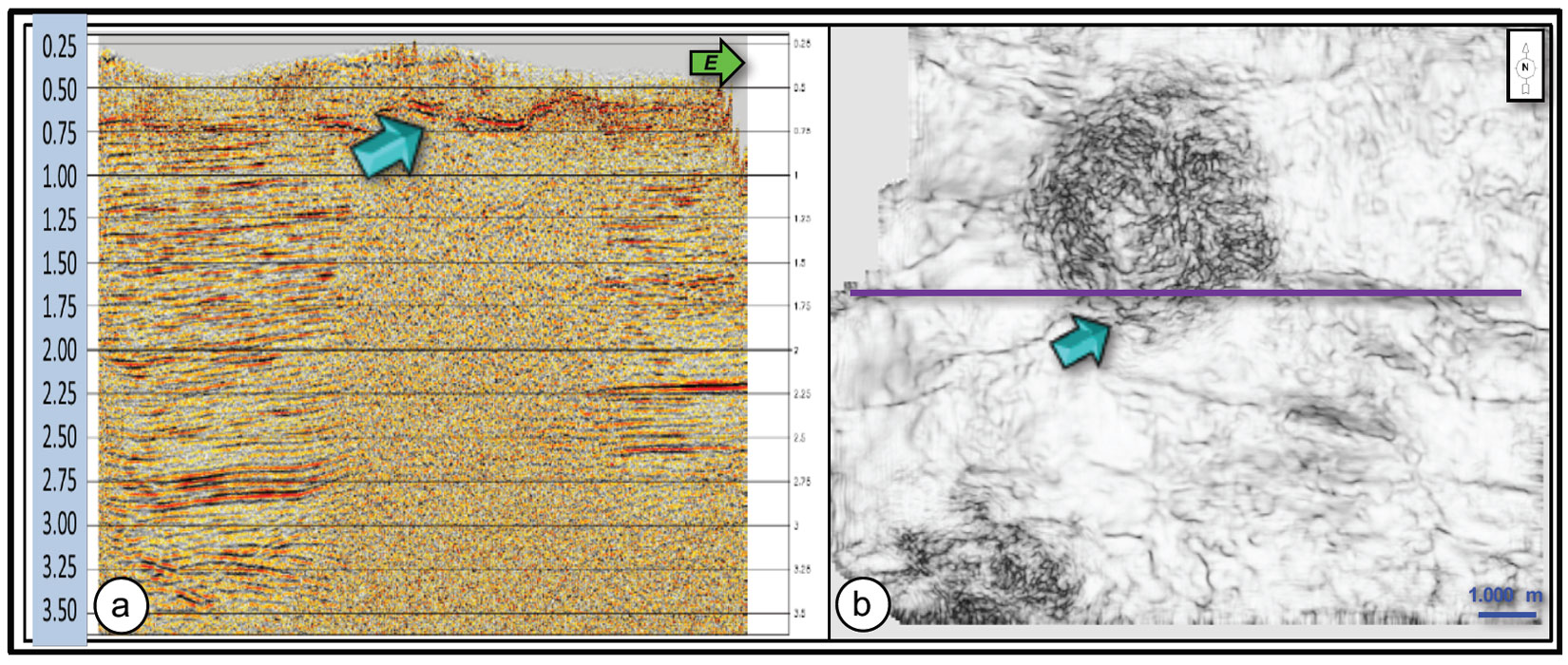
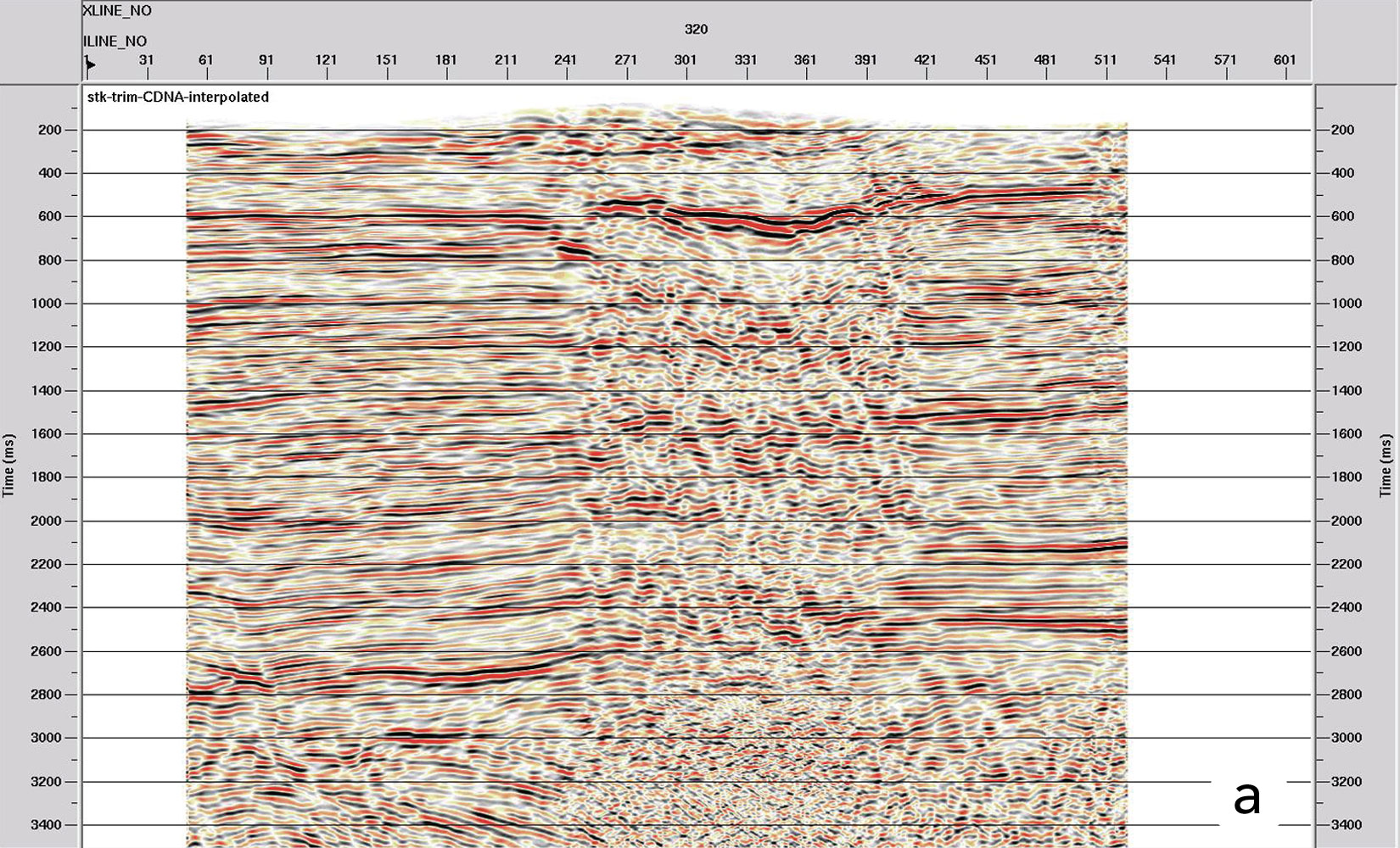
Unfortunately, the data produced by the 1997 3D was extremely variable in quality, deteriorating to an unacceptable level in the noise-prone areas. Cross-line 300 shown on Figure 2a) contains areas of no reflections (below 800 ms) over a considerable part of the line. And yet in other areas reflection quality is good and ties known well control. At one time, it was thought that a 5D interpolation algorithm might be able to generate the offsets and azimuths necessary to image reflectors amidst this noise. After using 5D interpolation, it can be seen that, while some reflectivity is evident, there is low confidence that much of the added reflectivity is geologically real and the improvement is insufficient for the interpreter needs.

The poor data areas become very evident when looking at time slices through a coherency cube. Figure 2b) is an example of such a display. Note the mottled appearance in two distinct areas. This correlates with the no-record areas on the in-line and cross-line displays. These areas are also consistent with well locations that show layers of basaltic sills at depths of about 500 meters.

Wells in the poor data area consistently contain basaltic sills in the 200 to 500 meter interval, but the sills are generally of erratic thickness and depth and had no correlation from well to well. In order to partially investigate the effect of such erratic sills on seismic records, a model was prepared with very high velocity segments in the shallow section (200-500 meters interval). These are intended to approximate the effect of erratic basaltic sills of variable thickness and position. Wave equation modelling was used to simulate the 2D shot records for 25 different shot locations.

Snapshots of the wavefields generated by the wave equation modeling are depicted in Figure 8. These snapshots are shown for a time 1.780 seconds after the source initiation. Downward propagating wavefronts appear as concave arcs while upward propagating reflections appear as convex arcs. Figure 8a) shows a wavefield for a source in a good data area where there are no basaltic sills in the near-field vicinity of the source.

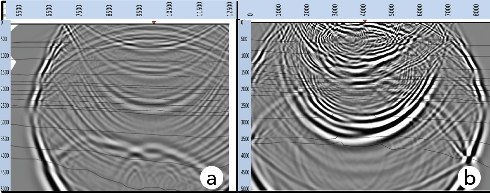
Figure 8b) shows reflections being generated at the deep targets, but as they rise towards the surface they are obliterated by much stronger chaotic events generated by diffractions from the erratic boundaries of the basaltic sills. Since the sills are erratic, then the scattered source-generated noise will be chaotic (i.e. random in space). Furthermore, the strength of the primary wavefield that transmits downwards through the layers of basalt is dramatically reduced due to the strong reflectivity of the basalt layers.

The very strong source-generated chaotically-scattered noise is generated locally by the strong diffractions and scattered waves that interact chaotically due to the random spatial locations of the variable near surface basaltic sills. The noise present dominates any weak reflection energy that may be passing through this part of the wavefield on its way back to the surface. Basically, weak deep reflection signals are lost in the presence of strong chaotic noise.

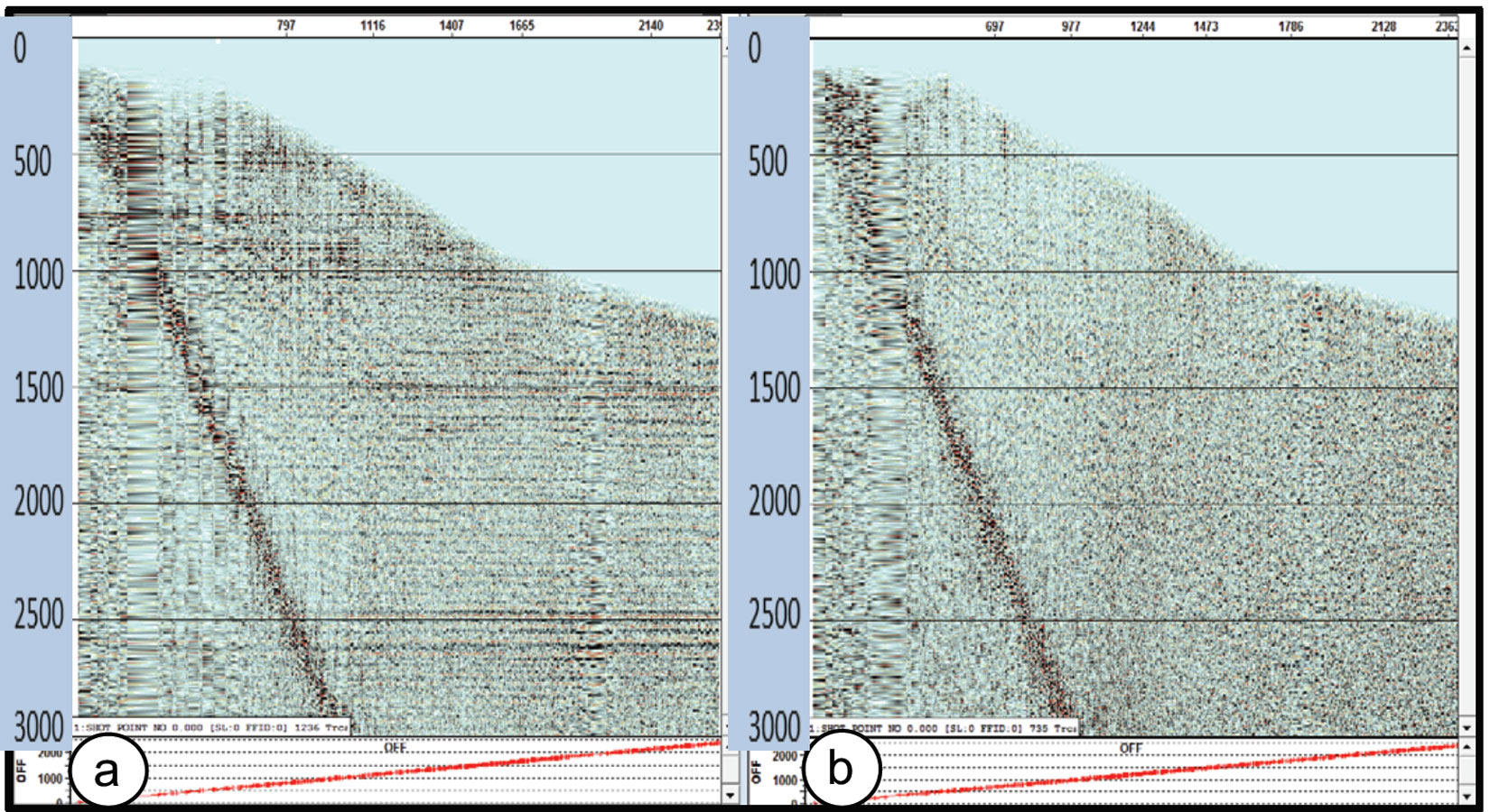
This phenomenon is clearly evidenced in Figures 9a and 9b which shows 5x5 bin super-gathers sorted by offset for two areas taken from the 1997 3D study area data volume. The gather on the left comes from a good data area in the northeast of the study area. The gather on the right comes from a poor data area where erratic sills of basalt are known to exist. Note that the correlated air blast (i.e. a strong surface wave) is evident on both records. However, deep reflections are not easily detectable in the poor gather.

Since this type of noise is not time-variant random, it requires an enhanced diversity of offsets and azimuths to provide unique and different measures of the noise within CDP gathers. The best way to improve stacked data quality in these conditions is to reduce line spacing in the 3D grid (Cooper, 2004).

The choice of line spacing is more of a continuum as represented in the following Equation. The values chosen between these limits should be based on an evaluation to the amount of chaotically-scattered, source-generated noise expected in the project area.

Where Ri=receiver interval, Si=source interval, SL=source line spacing, RL=receiver line spacing, Xmax=maximum useable offset for the zone of interest, Desired Fold= fold needed for the geophysical objectives

After careful study of the required parameters for imaging both signal and noise, two alternate sets of parameters were proposed. The parameters used for the 3D study area are: Ri=50 m, Si=50 m, RL=250 m, SL=350 m; the alternate 3D parameters are: Ri=48 m, Si=48 m, RL=192 m, SL=240 m; the recommended 3D parameters are: Ri=42 m, Si=42 m, RL=126 m, SL=168 m.

Sparcity refers to the number of sources between 2 adjacent receiver lines and the number of receivers between two adjacent source lines. The original 3D has a 5x7 sparcity, the alternate 3D has a 4x5 sparcity and the recommended 3D has a 3x4 sparcity. At the “M7” reflector levels using 1.670 m offsets the fold changes from 21.39 (5x7) to 47.53 (4x5) to 103.48 (3x4). The trace density changes from 34.223 (5x7) to 82.525 (4x5) to 234.223 (3x4) traces per square kilometer. It is better to quantify how the wavefield is sampled using trace density rather than fold (Lansley, 2004). Trace density is fold normalized by natural bin size.

Theoretical models using each of these parameters were generated. A variety of statistics including fold, largest offset gaps, offset and azimuth distributions, cross-plots of statistics, etcetera, only quantify various statistical properties and none of these tools tell how the stacked data will appear.

Reduction in line spacing will result in a significant increase in the cost of the program. Therefore, it is necessary to have a tool that helps to visualize what the potential benefit may be.

The super-gathers (Figure 9) from the original version recorded in 1997 show the character of signal and noise at every possible offset that can be expected in both a good and a bad data area. The proposed geometric models show the expected subset of recorded offsets in each bin. The “Data Simulation” tool is used to demonstrate how a stacked trace would appear for each bin.

In data simulation (Cooper and Herrera, 2014) a 3D model is used to determine what source-receiver offsets contribute to each bin. The right side of Figure 10 shows an example of the offset distribution of a typical 3D program with one bin hi-lighted. The distribution for that bin is reversed and expanded on the left side of this figure. Also on the left side of the figure is a representative CDP super-gather.

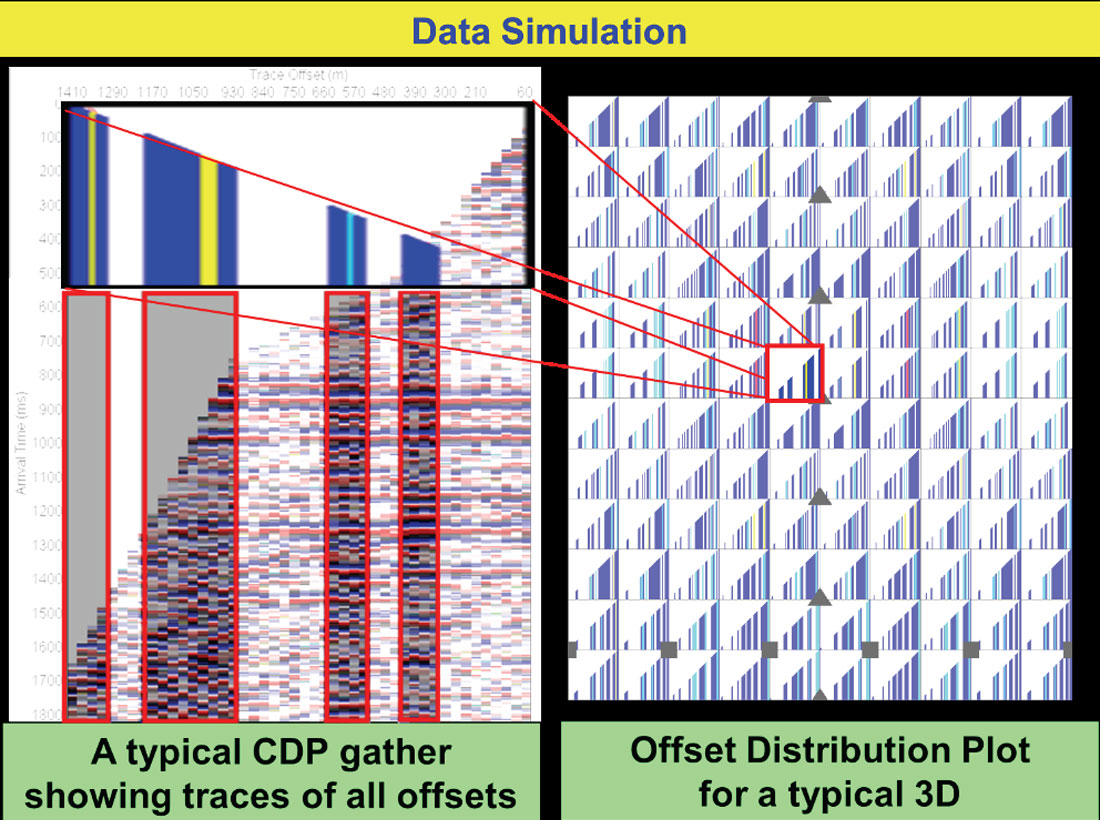
From this gather, only the traces that correspond to the offsets that will occur in the selected bin are selected. These are highlighted on the left side of Figure 10. The selected traces are then averaged together to produce a simulated stacked trace for the bin under consideration. Then it is necessary to move to the next bin, select traces that correspond to the offsets expected in that bin and use them to form a stacked trace for that bin location.

This process is repeated for the entire 3D study area to produce simulated data. Note that the same CDP reference gather is used to predict every stacked trace. Therefore, there will be no geologic difference from trace to trace in the simulated volume. The only differences from trace to trace will be how well the signal stacks constructively and how well the noise stacks destructively given that a different sub-set of all available offsets contribute to each bin.

Figure 11 shows the simulated stacked data for the three models described previously using the good data super gather. Note that where data quality is good, there is no significant motivation to use the more dense line spacing. Given that the estimated cost of the 3x4 model is about 2.33 times the cost of the 5x7 model, the additional cost is not justified by the moderate improvement in reflector continuity. Certainly, the denser grid reduces trace-to-trace variations in signal to noise ratio, but this would not result in a substantially different interpretability of the data volume.

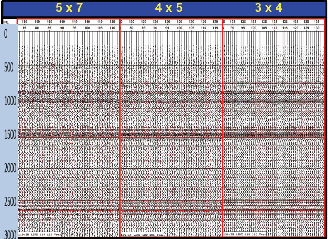
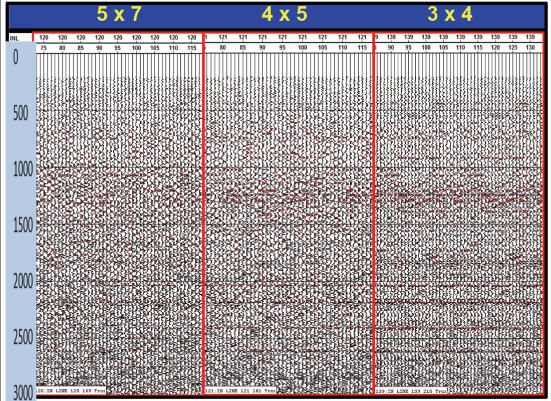
However, Figure 12 demonstrates the effectiveness of the more dense grids in areas where source-generated chaotically-scattered noise is known to dominate the raw records. In this case, the added offset diversity provided by the enhanced parameters clearly demonstrates a significant improvement in interpretability of the simulated data sets. This analysis gives the confidence to recommend the 3x4 sparcity even though the cost increase is substantial.

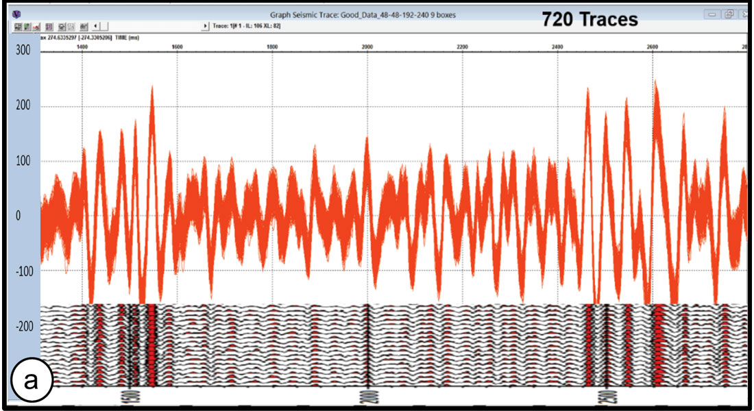
The traces contained in a 9 box area (a box is the area bounded by two adjacent source lines and two receiver lines) from the simulated volume using the 4x5 sparcity model were graphed. In Figure 13a), the 720 traces contained within those 9 boxes provide a consistent representation of several reflections. Note that a corresponding segment of the simulated stack is presented horizontally below the graphed traces.

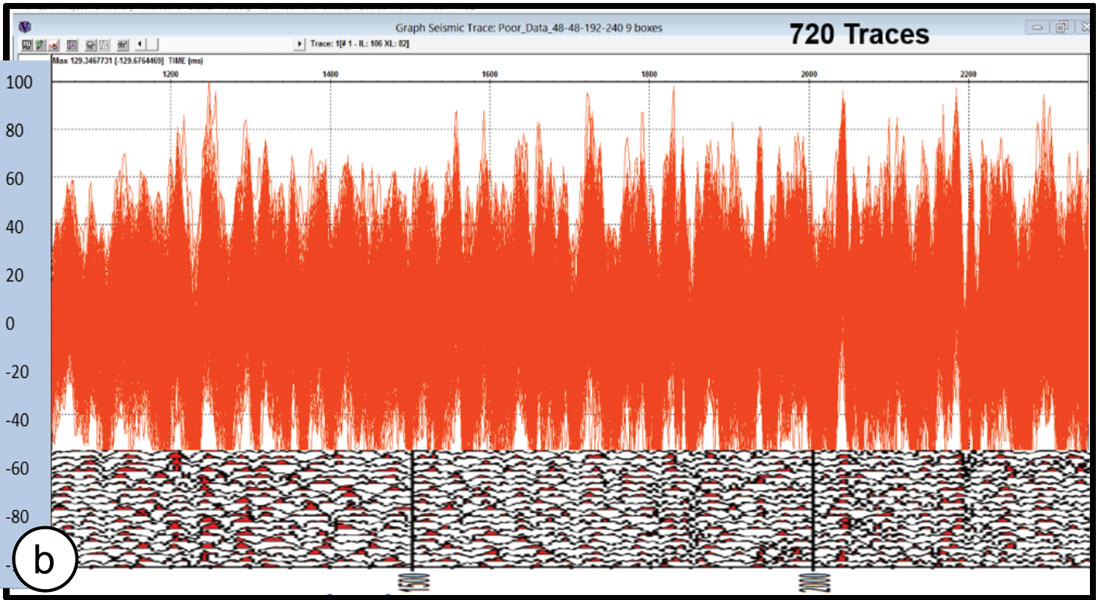
Unfortunately, this is not the case for the poor data area as seen in Figure 13b). The trace to trace noise level is so high that the reflectors are not discernable.

Using data simulation on a range of design geometries provides a clear visual representation of the expected benefits of the more costly designs. In this studied case, it appears that increased design density may be expected to provide the increase in data quality desired by the interpreter in the poor data areas. However, this is yet to be proven by re-acquisition of the survey using the recommended or alternate parameters.

This tool can be useful for an interpreter to visualize the optimization of line spacing (Cooper et al, 2014). Equation 1 provides a range of options while data simulation using local data samples helps to quantify the expected cost-quality benefit. It can indicate when a more dense survey is necessary for improved data quality and can also indicate when a sparser more affordable survey may be sufficient.

Conclusions

This paper presents options from the processing and the 3D design point of view as alternatives to overcome situations of seismic silence or great deterioration of the signal, as may be the case that is observed below the high velocity layers such as magmatic intrusive bodies.

It is important to be aware that design of 3D seismic programs should focus not only on measuring desired reflection signals, but also should evaluate the potential for scattered noise modes and allow for sufficient measurement of the noise components of the wavefield. Of course, the data simulation tool is a useful addition to help gauge the value of the final parameter selection.

Each particular case requires special attention to the conditions of the geological setting, topography, availability of equipment, environmental or legal limitations, etc. to clearly focus the objectives and to apply with certainty the concepts developed. This will help solve the situations of uncertainty, causing a significant improvement in the quality of the information and in the workflow results of the seismic interpretation. The interaction between the professionals involved is one of the keys to reach the objective of the work, both in the processing and in the design stage.

Acknowledgements

We thank Pan American Energy LLC, Mustagh Resources Ltd and DataSeismic Geophysical Services for allowing us to present this work. Thanks also to the developers and vendors of DirectAid, Vista and Tesseral software.