Scanning Calgary’s ‘Water Towers’: Applications of Hydrogeophysics in Challenging Mountain Terrain

• Alpine zones provide critical water storage for drier lowland areas like the Canadian Prairies. Groundwater plays an important role by helping delay the release of snowmelt to surface streams, but these storage processes have only recently been studied and are not yet completely understood.
• Traditional methods for hydrogeological investigations are not usually logistically possible in remote mountain areas. Geophysics offers a low-cost alternative and is useful for obtaining high-resolution datasets with large areal coverage.
• This article, using example data from our most recent project, illustrates how our research group uses geophysics to study mountain groundwater storage processes.
• Main take-aways for other practitioners of hydrogeophysics:
  • While logistically challenging, geophysics is an effective preliminary investigation tool for hydrogeological problems where direct sampling is not possible.
  • Surface observations and supporting measurements are key to making effective interpretations.
  • While some ambiguity may be unavoidable, using multiple methods greatly reduces the uncertainty in our final interpretations.

1 Introduction

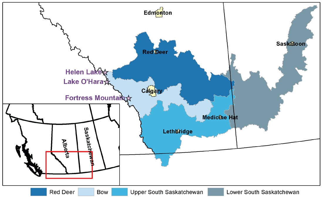
Among hydrologists, mountains are popularly referred to as the “water towers of the world.” Though only covering approximately 25% of the world’s land surface, they account for anywhere between 32% (Meybeck et al. 2001) and 60% (Bandyopadhyay et al. 1997) of water flow in all rivers. Moreover, a disproportionate number of people (37% of the world’s population) live in semiarid or arid areas that rely on mountain water sources (Viviroli et al. 2007). The South Saskatchewan River Basin in western Canada (Figure 1) is one such basin where mountain water resources play a major role. Spanning from the Rocky Mountains in southwestern Alberta to central Saskatchewan, the region has predominantly a semiarid, continental climate and is home to roughly two million people (Martz et al. 2007). While estimates vary, mountain zones contribute on average 38% of the annual river flow in this basin, varying seasonally by ±20% (Ashmore and Church 2001; Viviroli and Weingartner 2004). Hence, in western Canada, the metaphor of “mountain water towers” is appropriate.

However, despite the abundance of freshwater today, there are foreseeable challenges facing water resources in this region. For one, by 2009, 30% of the median natural flow in the region’s rivers was being consumed (AMEC 2009), and this proportion is expected to increase given population forecasts of over 3 million by 2046 (Martz et al. 2007). Moreover, late summer and autumnal flow in many rivers of the region has decreased since the 1960s because of higher average temperatures and decreased winter precipitation (DeBeer et al. 2016). Climatic changes are expected to lead to earlier spring melts, leading to further decreases in water availability during summer and autumn (Barnett et al. 2005; Tanzeeba and Gan 2012). However, reliable, quantitative forecasts of both demand and water supplies are difficult to make, meaning there is still substantial uncertainty in assessing the vulnerability to water shortages of communities downstream.

Our research group at the University of Calgary focuses on the supply side of the equation: mountain water resources. Specifically, we address the poorly understood role of groundwater in high-alpine basins. Up until the early 2000s, hydrologists often assumed that alpine catchments behaved like “Teflon® basins,” meaning that when snow melted or rain fell, it flowed almost immediately into streams (Clow et al. 2003). However, even thin layers of coarse, blocky sediments can store and help delay the release of precipitation to rivers. In a recent example, Hood and Hayashi (2015) found that 60-100 mm of all snowfall in one basin entered the groundwater, representing roughly 10-20% of all snow input. This in turn helped maintain stream flows in the fall and winter. Hence, if we want to make accurate forecasts of streamflow, we need to account for groundwater storage in our models.

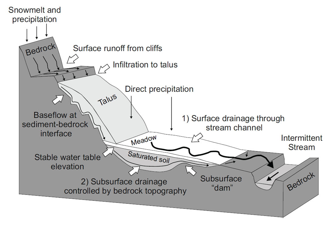
However, while we can measure how much goes in and comes out of the ground, making predictions is difficult because we do not understand the underlying processes very well. Many of our group’s studies from the past decade have focussed on questions such as, “What controls groundwater flow paths?” or “Where is groundwater stored?” For example, McClymont et al. (2010) showed that water flows primarily along the top of bedrock and that bedrock depressions can store and regulate water levels (Figure 2). Studies by Langston et al. (2011) and Mozil (2016) also showed that frozen ground can be an important interannual store of groundwater. Though these studies spanned only two field sites (Lake O’Hara in Yoho National Park and Helen Lake in Banff National Park), they give us early indications about important groundwater processes that we should account for when forecasting changing stream flows sourced from the Rocky Mountains.

Arriving at these conclusions was not easy because traditional methods of hydrogeological investigation (e.g. drilling wells, pumping tests, direct geochemical sampling) are not available to us at many of our field sites. This is partly because the sites are too remote to access with heavy equipment and also due to the regulatory constraints of operating within national or provincial parks. Hence, of the hydrologist’s standard toolkit, only weather data, surface sampling, and shallow auguring are usually available to us. For this reason, we often turn to geophysics for our hydrogeological investigations. These non-invasive techniques allow us to acquire laterally-extensive and low-cost data that can reveal geological structure and other information that are clues to the dynamics of groundwater flow.

This article aims to demonstrate how applied geophysics can lead to hydrogeological insights where more conventional investigation tools are difficult to apply. We will illustrate (using examples from our most recent study) what strategies are necessary for creating new, hydrogeological knowledge. First, we employ multiple geophysical methods that sample different petrophysical properties to accurately map the subsurface. Next, secondary observations, even when qualitative and sparse, are key to making reasonable interpretations. Finally, it is not always possible to arrive at a single “best” model, but narrowing the options to a small subset is still a desirable starting point for follow-up studies. While the motivation of our surveys was for answering scientific research questions, many of our insights about methodology of investigation should be of interest to practitioners of different disciplines. We hope to demonstrate that despite the logistical challenges of working in such difficult terrain, geophysics is an effective preliminary tool for streamlining later phases of a hydrogeological investigation.

2 Site description

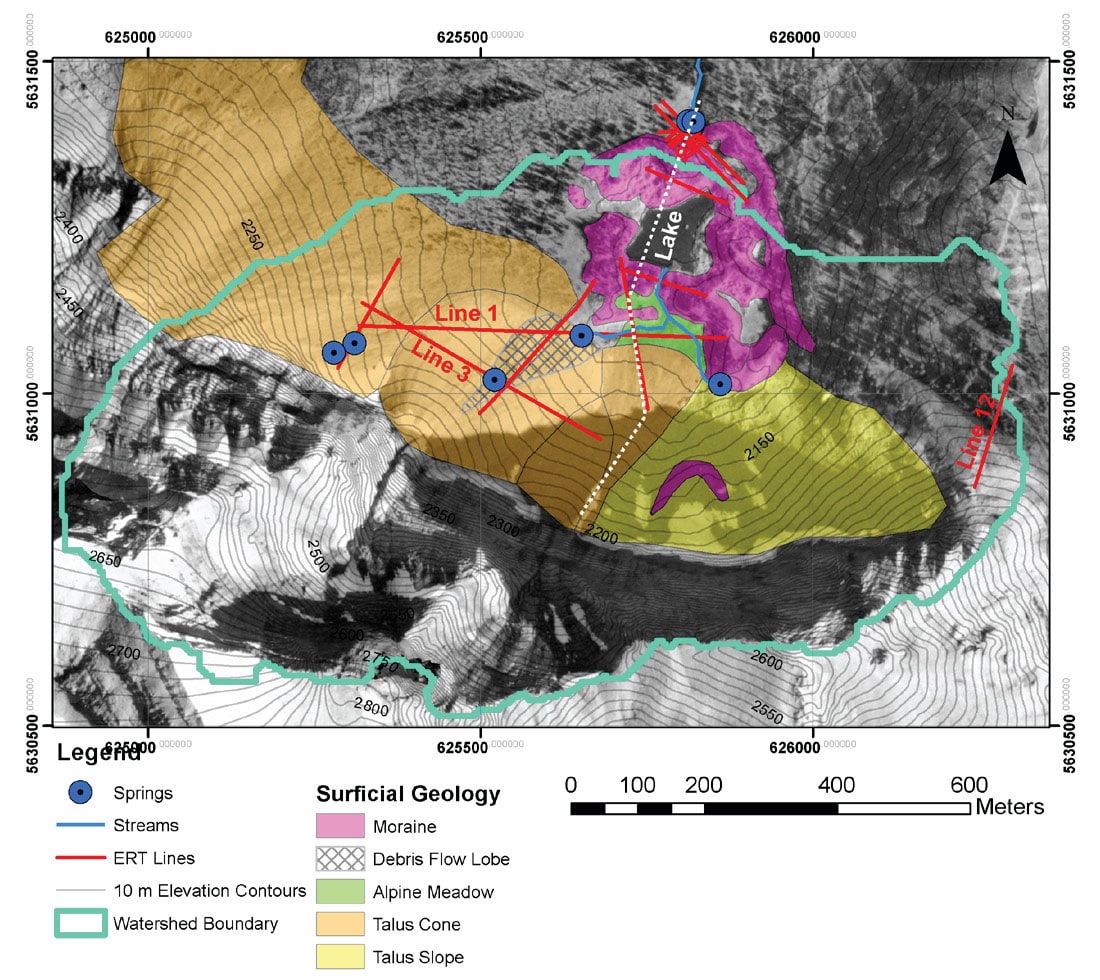
Fortress Mountain, located in Kananaskis Country, Alberta, Canada, is the site of our most recent hydrogeophysical study. Located in the Front Ranges of the southeastern Canadian Rocky Mountains at a former ski resort, our study focused on the area that drains into a small lake in the southeast corner of a cirque (Figure 3). This site was chosen for three reasons: 1) its complex geomorphology, 2) the obvious importance of groundwater, and 3) its contrasting bedrock composition.

First, the proximity of many different landforms in a small area make this site an appealing target for research. Partially vegetated talus cones and slopes lie at the base of the approximately 300 m tall headwall of this glacial cirque. At the toe of these slopes is a small meadow approximately 100 m by 50 m large. A complex array of moraines from previous glacial activity surrounds the main lake. With this variety, we can investigate how different landscape features convey and store water, and we can do so using relatively few geophysical lines.

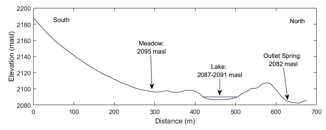
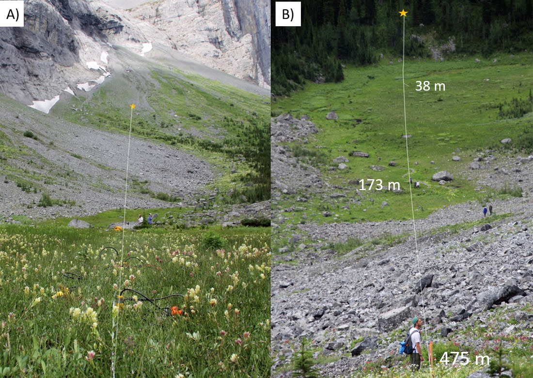
Second, there are obvious signs in this system that groundwater plays a significant role. There are multiple small springs that appear both at the base of talus slopes but also directly on the slopes. Similarly, immediately north of the lake, there is a large spring that flows year-round. Additionally, the lake is empty by late summer every year, yet there is no outlet stream to drain it. Figure 4 shows the relative elevations of these notable hydrological features. Though clearly important, the groundwater processes in this system are poorly understood and worth investigating because they sustain fall and winter stream flow.

Lastly, unlike previous sites in the Main Ranges, which are dominated by hard Cambrian quartzite bedrock of the Gogg Group, this site has younger, more heterogeneous bedrock composition. The base of the headwall corresponds to the Sulphur Mountain Thrust, a major regional fault (McMechan 2012). The headwall is composed of upper Devonian units: mainly the Palliser Formation (a competent limestone), with some weaker shale from the Banff and Exshaw Formations above that. The base of the valley is underlain by the Fernie Formation, a weak and highly fissile shale of the Jurassic Period. Given that bedrock played an important role in groundwater flow in our previous study sites, it is important for us to verify if our previous conclusions hold true when the bedrock here has such different properties.

3 Methods

3.1 Challenges of alpine geophysics

In our alpine hydrogeophysics work, we rarely have access to direct measurements to verify our geophysical interpretations, so we instead use multiple methods at the same locations. Our most commonly used methods (and the ones we used at Fortress Mountain) are: electrical resistivity tomography (ERT), seismic refraction tomography (SRT), and ground-penetrating radar (GPR). These techniques allow us to map electrical resistivity, P-wave velocity, and contrasts in dielectric permittivity, respectively.

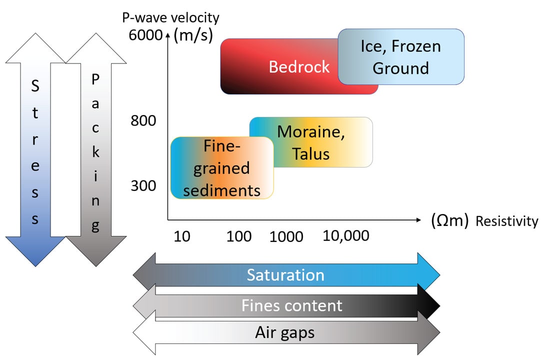
Acquiring multiple datasets allows us to use the complementary strengths of each method to improve confidence in our interpretations. For example, unconsolidated sediments and bedrock can be difficult to distinguish based on resistivity alone (Figure 5). Moreover, in alpine settings, there is often a thin, electrically conductive layer of water immediately above bedrock (see Figure 2) that tends to mask the presence of (even highly resistive) rock below it (Langston et al. 2011). Hence, using seismic refraction is critical for mapping the depth of the bedrock. By employing these three methods together, we can substantially reduce ambiguity in our interpretations about the hydrogeology.

Acquiring these data is not an easy task; getting equipment to site itself is challenging. On a limited research budget, helicopter delivery is out of the question. Furthermore, though we may get access to drive on some restricted roads, most equipment must be hand carried to the final location, meaning we must be parsimonious with how many data channels we use. However, Fortress Mountain is rather unique because we can drive to within one kilometre of our research area, making it easier to access than most locations.

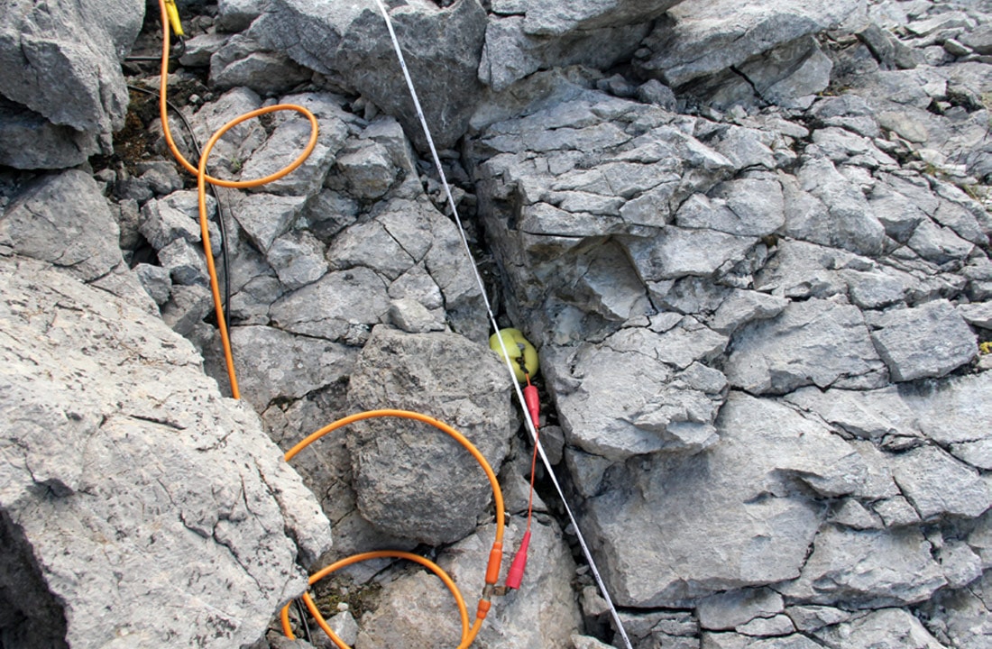
Beyond simply getting equipment to site, getting high-quality data is often a challenge. In ERT, one needs a good electrical connection with the ground, but rocky boulders on the moraines and talus of this site make it exceedingly difficult. To overcome this, we often take drastic measures to improve contact, including applying multiple electrodes in series, applying saltwater sponges (Figure 6), and even applying a kitty litter-water-salt mixture. This process of reducing contact resistance is usually the most time-consuming step in performing an ERT survey. Similarly, normal spike geophones designed for soil are useless on loose boulders. We instead use plate geophones on such surfaces, and weigh them down with rocks to improve coupling. Moreover, we do not have the luxury of using a push cart for GPR on such rugged terrain. Instead, we usually tie a rope between GPR antennae to help ensure a consistent separation length, and carry the antennae manually. While this terrain is challenging, these small tricks have helped us cope and acquire useable data.

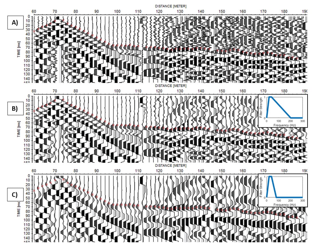
Despite these efforts, the signals received can be noisy. For instance, since we are limited to only very low-energy sources for SRT at most field sites, picking first arrivals at large offsets is difficult. This difficulty can be partly offset by some filtering to help us identify the correct pulse for picking first arrivals (Figure 7). With ERT, despite our best efforts, it can be practically impossible to reduce contact resistance below a desired threshold. However, we usually anticipate this, and hence often employ a very dense dipole-dipole acquisition sequence. While we take more measurements than would be necessary for most settings, choosing a longer acquisition time helps ensure that the data points we eventually reject do not constitute a debilitating proportion of our dataset. Hence, despite data quality issues, our acquisition and processing protocols help us combat these issues.

Lastly, working in remote locations leads to wildlife encounters. Normally this is only a minor inconvenience. Marmots and pikas often steal saltwater-soaked sponges, meaning that lines must be patrolled by our personnel during ERT acquisition. Moreover, the brightly-coloured cables can be chewed by curious critters, so cables cannot be left deployed overnight. Grizzly bears are a more serious hazard, especially in firearms-restricted parks. Luckily, at Fortress Mountain, there was only one sighting during all field work days and hence only minimal delays.

3.2 Acquisition parameters at Fortress Mountain

We used the Syscal Pro from Iris Instruments for our ERT acquisition. In short, current is injected into the ground with two electrodes, and the induced potential differences at other pairs of electrodes are measured to calculate the apparent resistivity of the ground. Our system allows for up to 72 electrodes per survey, with up to 10 simultaneous channels recorded per current injection. After setup, data acquisition is automated and usually takes one to two hours. At Fortress Mountain, we used an electrode spacing anywhere from 1 m to 8 m, depending on the resolution and depth of penetration required. We used the program Res2dInv (ver. 4.01.06) from Geotomo Software to invert measured apparent resistivity back to a resistivity model.

For SRT, we used the Geode system from Geometrics. A 5-kg sledgehammer struck on the aluminum plate was our energy source, and shots were spaced at every six channels (i.e. every 12 m with 2 m geophone spacing) and stacked 7-14 times to increase the signal-to-noise ratio. Geophone spacing ranged between 1.0 to 2.5 m, and 48 to 96 geophones were used per line. First arrivals were picked using ReflexW (ver 4.0) from Sandmeier Geophysical Research, and inversion modeling of seismic velocity was done using a code developed by Lanz et al. (1998).

Lastly, we used the PulseEkko Pro system from Sensors and Software to acquire GPR data. We used low frequency (50 MHz) antennae to increase depth of penetration and to avoid diffractions from large boulders in talus slopes. On the six reflection surveys collected, a constant 2 m antenna separation and 25 cm step size were used. These surveys were processed in ReflexW (ver. 4.0) using a standard workflow: dewow filtering, static correction, and exponential gain function. In addition, nine common midpoint surveys were collected at locations with strong reflectors present. Semblance analysis was used on these to get one-dimensional EM velocity models. We noted a strong correlation between EM velocity and resistivity. Hence, we used the inverted resistivity sections to compute a two-dimensional EM velocity model and thus convert GPR reflection sections from time-section to depth-sections.

Geophysical data were acquired over the course of two summer seasons. This included 19 days in July 2015 and five additional days of follow-up work in 2016. We have selected one line to present in this article (Line 1, see Figure 3). In addition, there were many other day trips for preliminary reconnaissance and collection of secondary data. Two of these data sets – hydraulic head data (a.k.a. piezometric data) from the meadow, and petrophysical measurements at known bedrock locations – are discussed in this paper.

4 Results

Line 1 is the longest of all the survey lines. At over 500 m in length, it begins on a moraine at the east end of the study area, crosses the meadow, passes over a spring at the base of a talus cone, and climbs up the talus to the west. Figure 8 shows photos along this line, and Figure 9 shows the three resulting geophysical processed sections. We will discuss these results in two parts: first looking at the talus, and then focusing on the meadow.

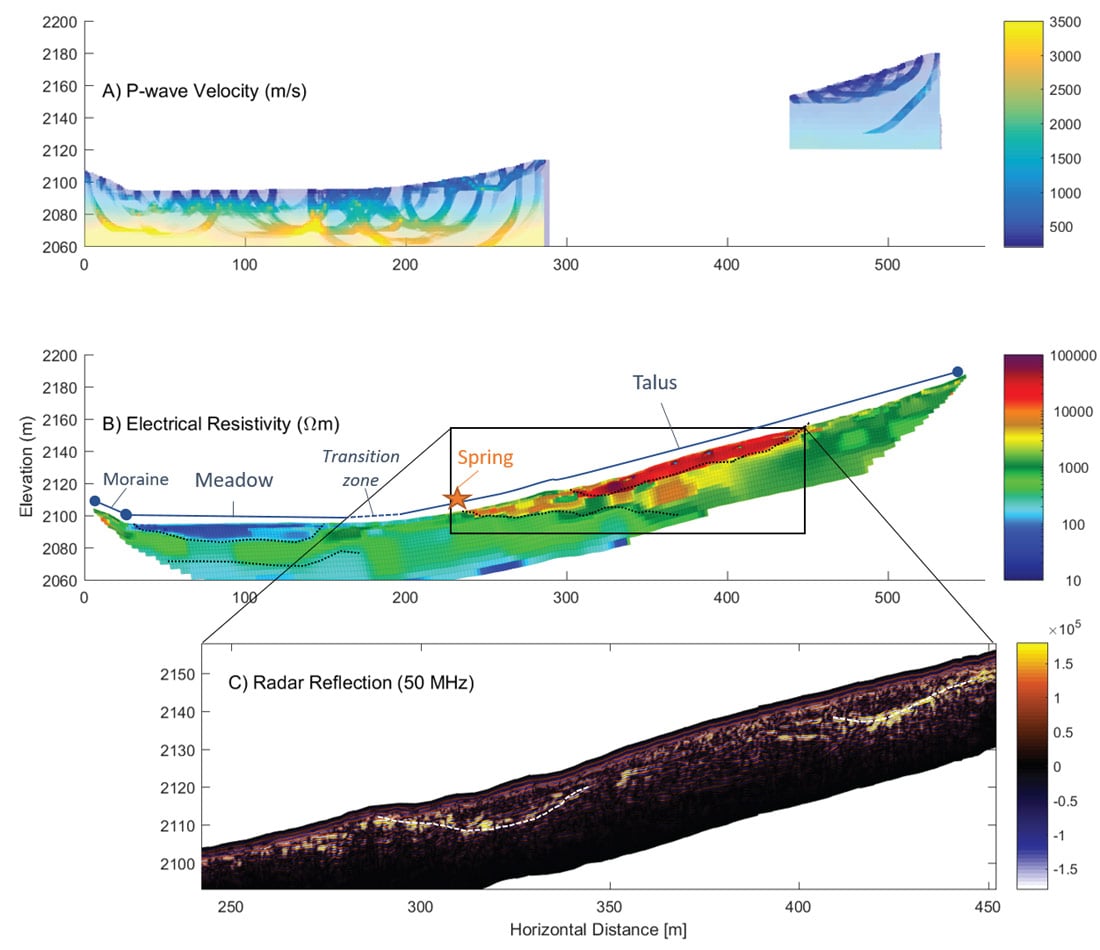
4.1 Talus

Within the talus, we identified three petrophysically distinct layers based primarily on resistivity: 1) large boulders with no fine-grained matrix (10,000-30,000 Ωm); 2) talus with large boulders and fine-grained matrix (3,000-5,000 Ωm); and 3) talus with large boulders, fine-grained matrix, and high water content (500-3,000 Ωm). This interpretation of the talus was partially based on surficial observations. As we moved upline, we noted an abrupt transition at 300 m from a mix of soil and boulders to large boulders that corresponds closely to a large increase in resistivity. Moreover, the spring at the base of the talus matched the location of another abrupt change in resistivity, at 220 m, from lower resistivity below the spring to higher resistivity above the spring. There were other springs and short-lived streams that ran between 450 and 490 m.

The other methods used help confirm this interpretation. First, the seismic refraction in this case helped confirm that the talus is unconsolidated material because P-wave velocities in these areas are generally below 1000 m/s. (In fact, a survey from the adjacent Line 3 shows that bedrock is 30-40 m below surface). The GPR supports it in two other key ways. First, the strongest amplitude reflectors (and hence largest contrasts in dielectric permittivity) occurred in locations where the 10,000-30,000 Ωm unit is directly above the 500-3,000 Ωm material. Furthermore, the EM velocity in the 10,000-30,000 Ωm and the 500-3,000 Ωm units were 0.13 m/ns and 0.10 m/ns, respectively. These strong reflections and decrease in velocity can be explained by some combination of a decrease in porosity, an increase in volumetric water content, or an increase in the dielectric permittivity of the fine-grained material. These possible explanations are consistent with the interpretation of the resistivity contrasts described.

4.2 Meadow

The resistivity and p-wave velocity models indicate that there are three distinct layers at the meadow. The properties of these are summarized in Table 1. The uppermost layer is easy to identify and is confirmed by soil auguring to be fine-grained, wet sediments.

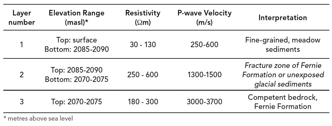
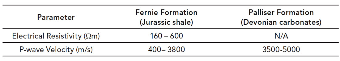
The lower two units were harder to identify without direct samples. To assist with interpretation, we collected one additional ERT and SRT survey, each conducted on the eastern ridge bordering this valley at locations where bedrock was exposed. Measurements of the petrophysical properties of the two main bedrock formations resulting from this additional survey are summarized in Table 2. Most notably, the surveys showed that the Fernie Formation, which is present as highly weathered, fissile regolith, has a wide range of velocities, and abruptly reaches a maximum velocity of between 3000-3800 m/s at depth. These additional data indicate that the high-velocity layer below 2070 masl at the meadow is clearly competent bedrock which has a resistivity value in the range of the Fernie Formation.

However, the additional data did not help us conclusively identify the middle layer below the meadow. With more intermediate velocities of 1300-1500 m/s, it may be weathered or fractured shale, but there are two caveats with this interpretation. First, given that the level of the lake is approximately 2089 masl (+/- 1 m), we expect the sediments below 2089 masl to be saturated. Since the resistivity of the water is in the range of 30-40 Ωm, we would expect a higher-porosity, fractured shale to have a lower resistivity than the competent bedrock, but the ERT model indicates the opposite. Second, in this complex glacial terrain, it may be plausible that other sedimentary units (say, an overconsolidated basal till) may not be visible at surface anywhere on site, but could match the resistivity and velocities modelled. Hence, we do not have a single interpretation that can explain all of our observations.

Despite these shortcomings, we can make some important conclusions about the hydrologic function of these layers. First, the range of velocities (1300-1500 m/s) indicates that this material is not consolidated. Moreover, in the summer of 2016, we monitored hydraulic head levels at three elevations in the meadow: in the small stream crossing the meadow (2093.6 masl), and at two different depths below surface (2092.4 and 2091.2 masl). We note that there is a strong vertical, downward hydraulic gradient, indicating that the stream above the meadow is losing water to the subsurface. Regardless of its true identity, our investigation has revealed that this layer is a porous, unlithified material that is hydraulically well-connected such that it is not a barrier to subsurface flow.

5 Discussion

5.1 New hydrogeological insights

One of the key insights of this project is the link between talus grain size distribution and flow path. In our previous studies, we observed that water would infiltrate rather quickly from the surface to the bedrock and that flow is concentrated in a thin layer above bedrock (Figure 2).

These new results show that the springs we see on the surface of the talus are tens of meters above bedrock, and that there is considerable heterogeneity in the distribution of grain sizes. Unlike the talus slopes at previous sites in the Main Ranges, where these slopes were dominated by large quartzite and limestone boulders with large air pockets in between, the mix of small shale fragments and larger limestone ones seems to lead to a denser packing and hence a lower hydraulic conductivity (i.e. fluids do not move as easy through it).

Our surveys revealed a similar contrast in how alpine meadows operate. Unlike the model proposed by McClymont et al. (2010), the fine-grained sediments do not sit directly on top of bedrock, but instead there is a thick package of 10-15 m of unlithified material immediately above bedrock. Hence, as with talus slopes, while the meadow here has a similar morphology at surface as seen in other areas we have studied, the controls on groundwater flow appear to be different.

These insights have important implications in how we should account for groundwater in watershed-scale modeling. A common approach to hydrological modelling is to divide a watershed into “hydrologic response units,” (Pomeroy et al. 2007) which are areas that are grouped together based on similar landscape features such as land cover, soil, elevation, slope angle, and aspect. (This means that, for instance, moraines may be grouped together and assigned similar hydraulic properties, as are meadows, and talus slopes). This approach has often worked in the past (Fang et al. 2013; Paznekas 2016) because alpine sediments were thin and do not vary considerably vertically and laterally at previous sites, or subsurface information was simply lacking. Our surveys at Fortress Mountain show that simply taking an inventory of sedimentary units at surface may be insufficient because there can be hydrologically significant layers below surface. Moreover, our study shows that applying this approach at regional level is not appropriate because landforms of similar genetic origin can have very different hydraulic properties between basins.

While we still lack the knowledge to construct these regional hydrological models, it does hint at certain large-scale trends. Paznekas and Hayashi (2016) compared the winter stream flows in watersheds across the Canadian Rocky Mountains. This steady discharge (known as winter baseflow) is fed almost entirely by stored groundwater. They noted that on a regional scale, watersheds with younger, sedimentary bedrock had a higher average winter baseflow than those with older, metamorphic bedrock. They speculated that this is because younger, less competent bedrock will be more fractured and have a higher porosity to store water, but also because bedrock characteristics have an indirect control on surficial geology. Our comparison of the talus characteristics here versus other watersheds is consistent with their hypothesis. Furthermore, if our interpretation of a thick weathered zone of bedrock below the meadow is correct, it would be consistent with this observed trend of more potential storage in basins with younger, sedimentary bedrock. While we still lack knowledge to predict how bedrock characteristics will quantitatively affect groundwater storage, our data supports this general trend.

5.2 Methodological considerations

This paper also illustrates some of the limitations of the use of geophysics for hydrogeological site investigations. First, using a single method would not have yielded such valuable information on its own, so in the absence of drilling, multiple methods were key. Moreover, we made use of additional surface observations – careful observation of change in surface cover, geophysics measurements at locations of known bedrock, and hydraulic head data – to increase the confidence of some of our interpretations. However, these being indirect observations, our data do not allow us to decisively identify the layer of material below the meadow.

Nevertheless, these surveys have given us valuable early insight into the hydrogeology of this site. Despite having very little previous knowledge, these areally extensive datasets have helped us identify hydraulically significant structures and reveal major trends. In a system this heterogeneous, this dense lateral coverage is especially important. Moreover, we did so at a very low cost. While some of our conclusions lack a high degree of certainty, they have constrained the set of feasible hypotheses to test and that will help focus our geochemical sampling, hydraulic monitoring, and numerical modelling. For instance, if we acquire funds for portable drilling equipment, sampling the material below the meadow would be the most valuable location to do so.

6 Conclusions

While challenging to implement, we have shown that geophysical surveys are a valuable tool for understanding the hydrogeology of an alpine headwater basin. Despite having minimal knowledge of the subsurface in the area, we have shown that there are: 1) complex flow paths controlled by uneven grain-size distribution in talus slopes; 2) a thick, unconsolidated unit under a meadow that is an important store of water; and 3) unlike previous areas, bedrock topography appears not to be the most important control of subsurface flow paths. These processes contrast with those observed in talus deposits and meadows in previous studies. This implies that to model groundwater accurately, one cannot use the same modeling approach for the same landscape feature in different basins. Moreover, our results indicate that a simple inventory of landscape units observed at surface is not always appropriate, and that there may be a link between bedrock geology and groundwater storage potential in a basin.

For other practitioners wanting to use geophysical methods for groundwater investigations, our study highlights key strategies for a successful campaign. First, we used multiple methods to reduce the ambiguity in our interpretations. Second, we made use of secondary observations to further reduce ambiguity. Finally, we were careful not to overstate the certainty of our data, and hence we maintained multiple conceptual models. Despite the limitations, we have narrowed our hypotheses to smaller set that can be tested with further sampling and numerical modeling work.

Acknowledgements

We extend great thanks to Fortress Mountain Resort for logistic assistance in helping us access this novel study area. We also thank our collaborators at the University of Saskatchewan’s Coldwater Laboratory led by Dr. John Pomeroy for getting us involved with this site. This work would not be possible without the contributions of all our field helpers, too numerous to name in this short space. We acknowledge the Norwegian Geotechnical Institute for sharing code for displaying ERT data. Finally, this research was funded by research grants from National Science and Engineering Research Council (NSERC), along with scholarships from the Canadian Society of Exploration Geophysicists (CSEG), the Canadian Exploration Geophysical Society (KEGS), and the NSERC Canadian Graduate Scholarship (NSERC-CGS) programs.