A Math-free Look at Azimuthal Surface Seismic Techniques

Many interpreters are interested in characterizing fractured reservoirs using 3D surface seismic data, and there are a variety of azimuthal techniques to extract this information from the data. However, once the results from two or more methods are compared the question may arise: why do the results from various azimuthal analysis methods differ?

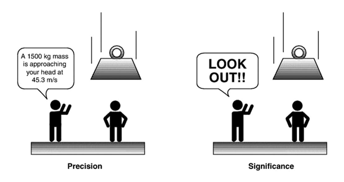
The following discussion is deliberately math-free. This is in response to an oft-heard request: “Please, no equations!” It is hoped that the loss of precision that comes from describing these ideas without using equations is compensated by a fresh perspective on their significance (Figure 1).

Spoiler Alert: The Short Answer

Why are the estimates of anisotropy often different depending on the azimuthal technique used? The short answer is:

The discussion begins with a brief review of the nature and scale of real-world fractured rock systems, and then considers three simplified frameworks to represent this complicated reality mathematically. We review the following azimuthal techniques for quantifying seismic anisotropy:

We then summarize how the anisotropy parameters output by each technique can be compared and formulated in terms of the three rock physics frameworks.

¹ S-wave amplitude differences may also be indicators of anisotropy; this method is not discussed here.Interested readers please see Reasnor (2001).

Fractures

Put simply, subsurface fractures usually occur in sets and are locally aligned in one dominant orientation. The fracture aperture size is typically in the ballpark of hundredths to tenths of a millimetre, and the distance between adjacent fractures is much greater than the fracture aperture. Fracture intensity is less than 0.75 fractures/m for very sparse sets, and may exceed 10 fractures/m for very crowded sets. In contrast, seismic wavelengths are typically tens and hundreds of metres, which means that we can model a fractured zone as a seismically anisotropic solid.

Fractures Can Make Rock Seismically Anisotropic

Fractures act as speed bumps – they can slow seismic waves traveling perpendicular to them, while waves traveling parallel to them are not really affected. By characterizing the seismic anisotropy, the goal is to work backwards to estimate physical properties of interest such as fracture intensity and orientation (where are the speed bumps and which way are they oriented).

To Describe Anisotropy: Models of Fractured Media

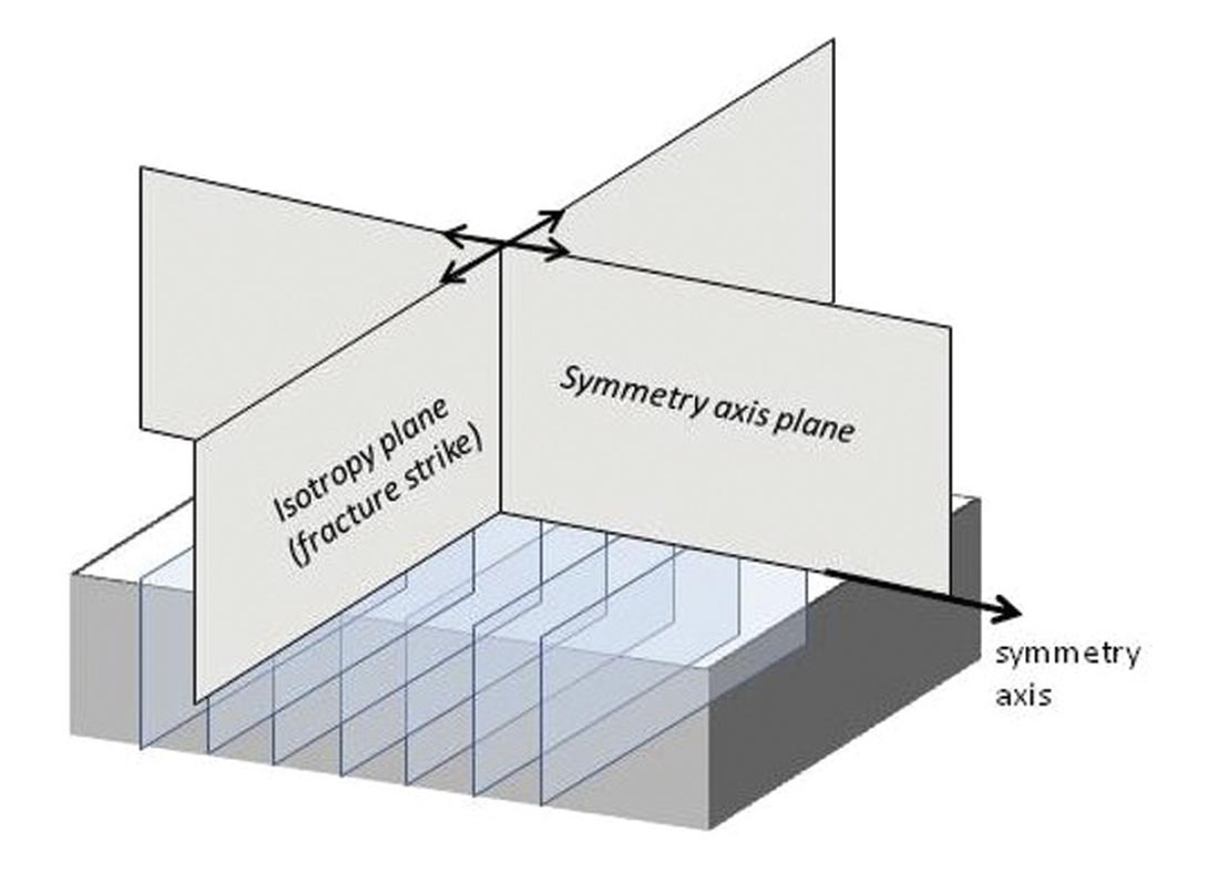
When we discuss seismically anisotropic media, we need some way to characterize the physical features and their directional nature. One quickly sees that the complex irregularities of the real-world situation – a porous rock with vertical-ish cracks and fractures – are not easily portrayed by equations. To enable a mathematical description, we turn to a simplified representation of reality. We consider the reservoir rock as having a set of vertical fractures – a horizontally transverse isotropic (HTI) medium (Figure 2) – and explore three rock physics frameworks for explaining HTI anisotropy. While these mathematical models might at first impression looked complicated, they are all based on physical parameters (velocities, fracture aperture, etc.) and they set a foundation for interpreting the anisotropy parameters and for the ‘Comparing Methods’ section of this article.

1. Thomsen-style Model: Vertical “Layers” of Anisotropic Media

To characterize the directional differences in transversely anisotropic media, five elastic parameters are needed: Young’s elasticity moduli parallel and perpendicular to symmetry, and Poisson’s ratios parallel, perpendicular, and typically at 45° to bedding (that is, 45° to the vertical symmetry axis). Thomsen considered VTI horizontal anisotropic layers (such as shale beds) and showed that for weakly anisotropic rocks, these five elastic constants can be recast into more geophysically accessible parameters: P- and S-wave velocities along the vertical symmetry axis, and three dimensionless fractional parameters γ, ε, and δ. How far these Thomsen parameters deviate from zero characterize the relative strength of anisotropy.

By performing a coordinate rotation, Rüger extended the VTI parameterization to the HTI case (such as our set of vertical fractures), giving the Thomsen-style anisotropic parameters γ^(v), ε^(v), and δ^(v) (the superscript ^(v) denotes that the vertical velocities are used as reference velocities). γ^(v) represents the fractional difference between fast and slow S-wave velocities, and is sufficient to determine shear wave velocity at any direction of travel. For compressional waves, the wavefront may be non-elliptical: Pwave velocity becomes a function of both incidence angle and azimuth. To describe it fully, two parameters are needed: ε^(v), which is the fractional difference in fast and slow velocity for Pwaves travelling horizontally through the HTI zone, and δ^(v) which describes P-waves travelling obliquely (that is, at intermediate incidence angles and not in the isotropy plane). It is important to note that we cannot get ε^(v) directly from surface seismic data (because waves travelling horizontally – that is, having incidence angle of 90 degrees – are unlikely to be recorded by surface receivers, even those at the farthest sourcereceiver offsets in the survey). We have to use data from intermediate incidence angles, hence Thomsen’s anisotropy parameter δ^(v) is key to characterizing anisotropy for surface seismic data.

The physical meaning of δ^(v) is a bit elusive to unpack². It turns out to be a very important parameter for understanding the fractured rock, and we will expand on the significance of δ^(v) in the following section, in the context of fracture weaknesses.

2. Linear Slip Theory Model: Fractures as Parallel Planes of Weakness Inside a Host Rock

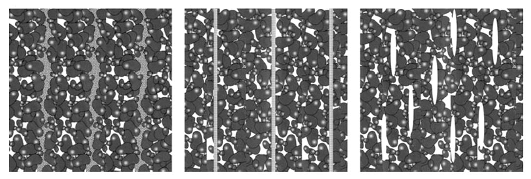
While Thomsen-style parameters characterize anisotropy, they do not make direct reference to fracture properties, consequently it can be useful to look to more specific models. Linear Slip Theory (LST) is a model that describes fractures as surfaces inside an isotropic host rock (Figure 3).

LST parameterizes the fractured rock in terms of compliance; compliance is the inverse of stiffness. The total elastic compliance of the fractured rock is the sum of the compliance of the background non-fractured rock plus the excess compliance due to the fractures.

The fractures can be parameterized in terms of fracture compliance, or alternatively, fracture weaknesses. This second parameterization describes how fractures weaken a background isotropic rock, and has the advantage of being a fractional value. The stiffness matrix of the HTI media is expressed in terms of elastic parameters λ and μ of the isotropic host rock, and the normal and tangential weaknesses δ_N and δ_T of the fracture system³ (δ_N means normal to the plane of the fractures; δ_T means along the plane of the fractures⁴).

Normal and tangential weaknesses convey how much of the strain of the fractured rock system is taken up by the fractures (the strain is the displacement due to a normal or tangential stress or force). The normal fracture weakness δ_N describes how a fractured rock will react to a normal force (a force acting to push the fracture surfaces together) and will be affected by fluid content (a waterfilled crack is more difficult to compress than a gas-filled crack), crack density and aperture. The tangential fracture weakness δ_T indicates how fractured rock will react to shearing force (a force trying to slide the fracture surfaces across one another) and is unaffected by fluid content. These dimensionless parameters range from 0 to 1; a fracture weakness of 0 means the fracture has no influence on the stiffness of the rock, 1 means that the rock falls apart (has no normal or tangential stiffness).

Note that when the LST model is assumed, it is possible to express Thomsen’s anisotropy parameters as scaled versions of normal and tangential fracture weaknesses (the equations are provided in the Appendix). As one might expect, γ^(v) – which describes shear wave velocities – is a function of only the tangential fracture weakness. To understand more fully the physical meaning of Thomsen’s δ^(v) parameter, it is instructive to observe that while ε^(v) is a function of only the normal fracture weakness (remember ε^(v) describes the compressional horizontally-traveling velocities), δ^(v) – which describes the P-wave anisotropy at oblique incidence – is a function of both normal and tangential fracture weaknesses. This presents itself on surface seismic data as variation of P-wave velocity with azimuth and incidence angle, and is a reason for the complicated P-wavefront shape.

² Thomsen's anisotropy parameter δ^(v) is not simply a scaled ε^(v), it is a physical parameter: a non-intuitive combination of stiffness coefficients from the rock’s linear elasticity matrix that are needed to describe P-wave velocity at oblique incidence angles.

³ Unfortunately the literature has used the Greek letter delta, δ, for weakness. This is different from Thomsen’s anisotropy parameter δ. Some literature uses the upper case, Δ, for weakness, but as this has a previous connotation in geophysics as meaning the change in a property across an interface, we will stick with δ_N and δ_T for normal and tangential weaknesses of the fracture system, and δ^(v) for Thomsen's delta anisotropy parameter in HTI coordinates. No wonder there arises a plea for equation-free summaries!

⁴ δ_T can be further decomposed into tangential-vertical ( δ_V ) and tangential-horizontal (in the fracture plane) ( δ_H ) weaknesses, but to keep things simple, in this article we disregard this complication.

3. Hudson’s Model: Fractures as Aligned Isolated Pennyshaped Cracks Inside a Host Rock

Hudson’s penny-shaped model is conceptually simple to understand and has been experimentally verified. But it imposes more restrictive assumptions than LST.

Hudson’s model considers fractured rock as a single set of parallel penny-shaped cracks in an isotropic host solid (Figure 3). The cracks are ellipsoidal shaped (oblate spheroids) and the cracks are isolated –meaning that the model does not account for possible fluid flow between the cracks.

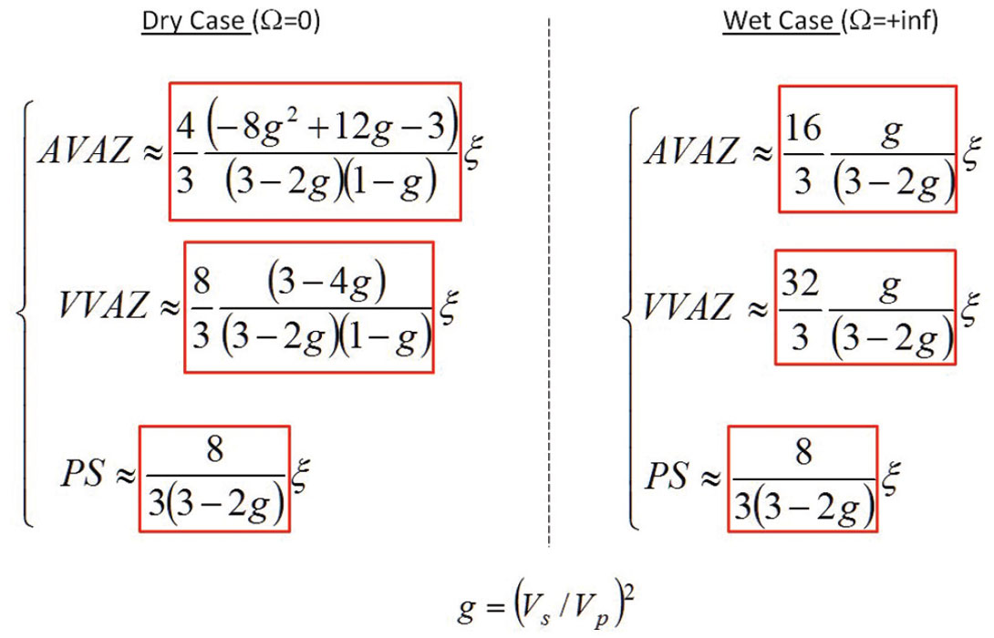
Hudson’s penny-shaped crack model parameterizes anisotropy in terms of crack density ξ, the number of cracks per unit volume, and a fluid term k representing the stiffening effect of the fluid content. It is possible to isolate the fluid effect and the influence of the aspect ratio (crack shape) with a single variable which we call Omega, Ω. When W approaches Ω, we have the dry case (compliant); when Ω approaches infinity, the fluid-filled crack case (stiff).

Note that compared to Thomsen-style parameterization, LST and Hudson’s models:

• narrow the solution space (by making more assumptions on the fracture set);
• directly relate anisotropy parameters to fracture properties; and
• can be parameterized with two variables instead of three.

LST has been our “preferred model” in parameterization so far because of the intuitive understanding of weaknesses that it offers, and because it does not require the strong assumption of penny shaped cracks.

Estimating Seismic Anisotropy Using Azimuthal Techniques

Now that we have reviewed how seismic anisotropy can be represented by these three simple models, we turn our attention to ways of measuring anisotropy from the seismic data. To estimate any rock property which has a directional quality, one needs to account for the direction of travel of the seismic waves. In 3D surface seismic data, this means that, at every bin within a 3D survey, one must extend the usual prestack analysis to account for azimuth.

Travel Time-based Methods

Shear-wave Splitting⁵ Technique

If the 3D survey was recorded using multicomponent receivers, azimuthal analysis of the mode-converted (PS) data can provide estimates of anisotropy.

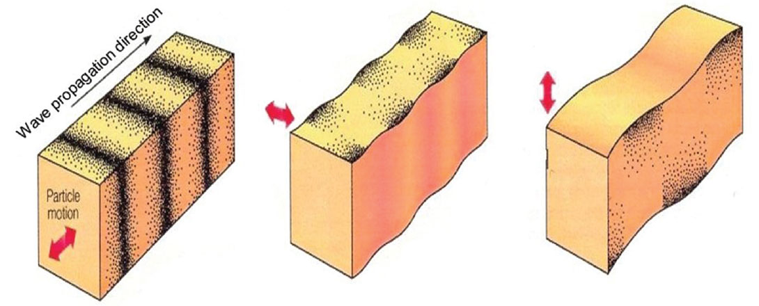
While compressional waves (P-waves) have particle motion in the direction of wave propagation, shear, or S-waves have a particle motion orthogonal to the direction of wave propagation (Figure 4). In the simplest case, S-wave particle motion is polarized in two directions: horizontal and vertical.

A set of parallel fractures, like our HTI vertical fractures, will act as a polarizing filter on a shear wave travelling through the fractured zone. Roughly speaking, the fractures split the converted S-wave into a fast S1 component - aligned parallel to the fracture set - and a slow S2 component - perpendicular to the fracture set.

Following appropriate 3C data processing, estimates of fast PS1 polarization and PS1-PS2 time delay may be derived. This operation is performed in a layer stripping manner. This analysis is automated and repeated at every spatial location. Symmetry axis and anisotropy magnitude attributes for the target zone are output. The anisotropy magnitude delivered by the Shear-wave Splitting technique is directly related to Thomsen’s γ^(v).

VVAz: Variation of Travel Time with Offset and Azimuth Technique

VVAz, also known as Azimuthal NMO, examines variation in travel time (velocity) with azimuth to characterize the anisotropy. With the introduction of aligned fractures, the rock structure can no longer transmit compressional waves equally well in all directions. The fractured rock system’s incompressibility is diminished, hence the P-wave velocity is reduced (recall our speed bump analogy). Azimuthal NMO methods simply try to describe how P-wave velocity varies with direction of travel.

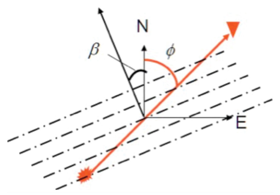
For short recording offsets – less than or equal to the reflector depth – the variation in NMO velocity with azimuth can be described by an ellipse. This velocity ellipse is a simplified model, characterized by the major axis, V_fast; the minor axis, V_slow; and the azimuthal orientation of V_fast. For most rocks the fast velocity corresponds to the rock matrix, and so the orientation of V_fast is parallel to the fracture strike. The ratio of the two velocities provides an estimate of the magnitude of the anisotropy. The anisotropy magnitude delivered by VVAz is directly related to Thomsen’s δ^(v).

The analysis of effective anisotropy gives V_fast and V_slow averaged down to the target and is typically used to correct for azimuthal moveout in the data and to improve the imaging. Once the cumulative influence of layers above is removed, then a zone-specific analysis of the anisotropic zone of interest (our set of vertical fractures) is conducted through the use of interval velocities.

⁵ Shear-wave Splitting is more properly called shear wave birefringence.

AVAz: Amplitude-based Methods

We discuss the following amplitude-based methods:

• Rüger-style Azimuthal AVO (AzAVO)
• Azimuthal Fourier Coefficients (Az FC)
• Azimuthal Fourier Coefficients Elastic Inversion (Az FC Inv)

Near offset Rüger-style Azimuthal AVO (AzAVO) Technique

Near offset Rüger-style Azimuthal AVO is the traditional method that most people think of when one talks about “Azimuthal AVO”.

Fractures lower both Vp and Vs, but by differing degrees. This difference in (Vp/Vs)parallel-to-the-isotropy-plane to (Vp/Vs) perpendicular is what drives an azimuthal AVO response. The amplitude gradient will vary with direction, and the largest variation will be between the AVO responses parallel and perpendicular to the isotropy plane.

The near offset Rüger-style Azimuthal AVO technique is based on Rüger and Tsvankin’s (1997) near offset (two-term) Azimuthal AVO equation which predicts that at the interface of an isotropic medium overlying an HTI medium, the reflection’s AVO Gradient (B) varies with azimuth in an elliptical fashion between two simple extremes: parallel to the isotropy plane and perpendicular to it.

If there is no anisotropy then the AVO Gradient is the same in all directions: B_iso. If there is anisotropy, then the AVO Gradient varies with azimuth; in the direction of the symmetry axis, the AVO Gradient is the sum of B_iso and B_ani at that azimuth. B_ani is a measure of how much the anisotropy perturbed the isotropic AVO response.

However, and this is a very large ‘however’, the axis of symmetry estimated by Rüger-style AzAVO carries with it an ambiguity of 90° (for example, “The fracture strike is at a bearing of either South or West, but we cannot tell which”). Why?

Mathematically, the least-squares solution of the near offset Rüger-style AzAVO equation gives the magnitude of B_ani, but it cannot tell us the sign. The equation has a non-unique solution: two answers fit the data equally well. This uncertainty in the sign of the anisotropic gradient B_ani translates into a 90° ambiguity in AzAVO’s estimated axis of symmetry (and hence the fracture strike, which is perpendicular to the symmetry axis).

The outputs of AzAVO are the azimuth of the axis of symmetry (with a 90° ambiguity), and the Anisotropic Gradient, Bani, which describes how the AVO gradient varies with azimuth. It is important to note that the interpretation of Bani is not straightforward: it is a reflectivity parameter (a measure of contrast from one layer to another) and it is a weighted difference of γ^(v), and δ^(v). It is only when assuming Hudson’s model that B_ani may be interpreted as a direct indicator of fracture density.

Azimuthal Fourier Coefficients Technique

Azimuthal Fourier Coefficients are also an Azimuthal AVO interface analysis, but the math is handled in a new way. As well, unlike Rüger-style AzAVO, Az FC does not require the assumption of isotropic overlying HTI media, and it is not a near offset approximation; an approximation which, as pointed out by Goodway et al. (2006), can have a strong influence on the results.

For HTI media, at any incidence angle, amplitude variation with azimuth is repetitive (Figure 5). One can therefore calculate a Fourier transform of amplitude variation with azimuth at any particular angle of incidence to decompose the waveform into a Fourier series.

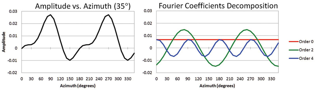
The bulk of the information is captured in the first few Fourier coefficients (FCs) of the series; indeed, coefficients higher than fourth order can be neglected. The properties of the Fourier transform allow AVO and AVAz to be treated as separate problems: the n=0 FC is equivalent to the classic three-term AVO expression, the AVAz part is portrayed by the 2nd and 4th FCs.

The anisotropic gradient, B_ani, and the symmetry axis can be obtained using the 2nd FC at just one incidence angle (!), but with some ambiguity in the symmetry axis. By including more angles of incidence and the 4th FC, the symmetry axis ambiguity can be resolved and an improved estimate of the B_ani obtained.

It is important to remember that with conventional AzAVO methods, one cannot be sure how much of the amplitude variation is due to fracturing and how much is due to isotropic AVO. One of the key advantages of the Az FC method is that since we are examining one incidence angle at a time, we are able to separate the AVO and AVAz and therefore avoid cross-talk between the two.

One can push forward and derive fracture parameters, such as weaknesses, which would be more straightforward to interpret than B_ani. However these parameters would still be reflectivity parameters, this is one of the important motivations to continue on to a true azimuthal inversion.

Azimuthal Fourier Coefficients Elastic Inversion Technique

Az FC Inversion uses all the Azimuthal Fourier Coefficient volumes (simultaneously at each incidence angle) as input and computes a deterministic geologic fractured model that best matches the available data. As well, the solution complies with user-defined physical constraints, such as lateral continuity or realistic weakness values.

One important input is the initial model. It is now possible to input a spatially variable Vp/Vs volume which can be derived from a standard isotropic elastic inversion. For the fracture parameters initial model, we typically start from the isotropic case where δ_T and δ_N = 0 or introduce a background trend model.

In addition to integrating all the available data, the biggest upside of the method is that it solves for layer properties. In comparison to interface reflectivity analyses, the inversion process inherently brings a more stable and objective solution, simplifying the interpretation.

The Az FC Inversion approach outputs an unambiguous orientation for each layer, and can be directly parameterized to output fracture properties like normal and tangential weaknesses. From there one can easily remove the anisotropy to correct elastic parameters (such as Poisson’s ratio) to their true isotropic value.

Comparing Methods

Resolution

When comparing results, it is important to remember that AVAz methods results have the resolution of the seismic bandwidth; VVAz is lower; S-wave Splitting generally lower still, due PS data quality (Figure 6).

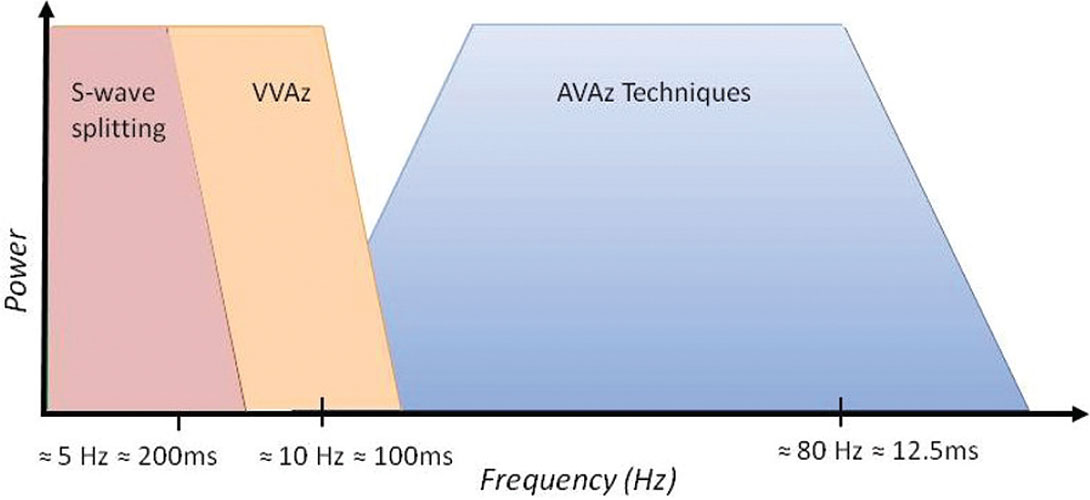
VVAz and S-wave Splitting convey information about trends, where AVAz techniques will not capture these trends but local deviations. Usually when we discuss resolution we are concerned with having sufficiently high frequencies to resolve details, but it’s the low frequencies that are needed to establish the background trend. This becomes important when deriving quantitative measurements like stresses, as pointed out by Dave Gray (Gray et al., 2012), and calibrating the results to other measurements.

One should keep in mind the inherent differences in resolution of the various methods when interpreting the outputs. For example, the low frequency measurements may give information about regional stresses but cannot be expected to reveal local variations, just as the high frequency measurements may reveal localized variations in the stress field or local natural fractures but ought not to be interpreted as regional trends. These differences in resolution might be why seismically-derived stress estimates which invoke AVAz in their workflow don’t always show the regional dominant stress.

Azimuthal inversion can potentially be used as a data integration tool; an initial model can be provided to fill the missing low frequency. The logical next step will be to use VVAz and S-wave Splitting for the background information and input this model for AZ FC Inversion. This approach is still under testing but opens the door to more accurate quantitative analyses.

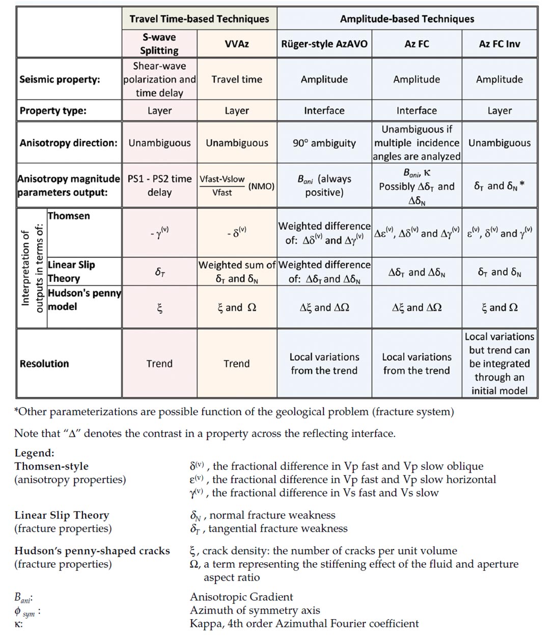
Azimuthal Techniques and Models of Fractured Media: Summary Table

The above azimuthal methods each output two basic anisotropy parameters: axis of symmetry (anisotropy direction), and magnitude (how anisotropic is it). These can be interpreted in terms the rock physics models. It is important to note that the models can be formulated in terms of each other (the equations illustrating this are shown in the Appendix).

The table helps us understand when the results from the various azimuthal techniques may be compared. For instance, when formulated in terms of LST we see that anisotropy magnitude measured by S-wave Splitting relates directly to tangential fracture weakness δ_T, and for VVAz it relates to a weighted sum of δ_T and δ_N. Since the weakness values are always positive and the methods have the same property type and resolution, the results from these two techniques could potentially be compared. But one should not expect the result from Rüger-style AzAVO method – being a weighted difference of δ_T and δ_N in LST formulation – to be always comparable with the results from VVAz and Shear-wave Splitting methods.

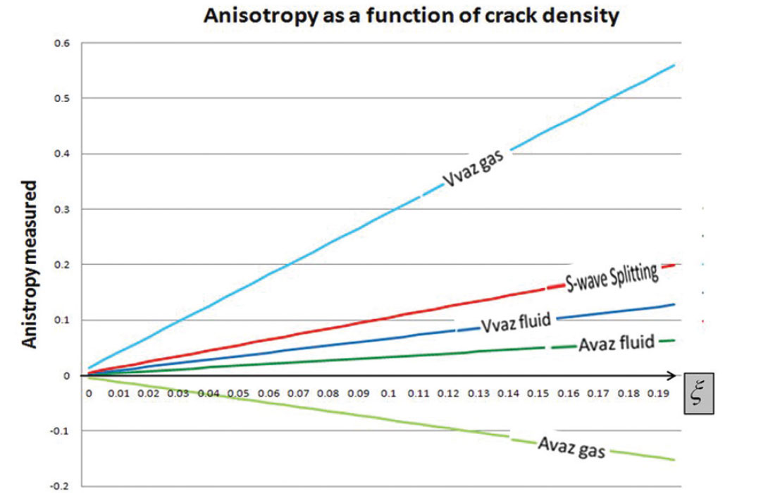
If we assume Hudson’s model (fractures are aligned isolated penny-shaped cracks) and we assume isotropic overlying HTI media, then all techniques become comparable and linearly scaled to the crack density. (Just remember that this model places the most assumptions, and there are inherent resolution differences between the methods.)

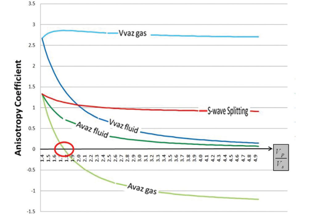
In other words, assuming Hudson’s model, the anisotropy parameters output by each method are scaled versions of the crack density, ξ. Each method scales the crack density differently, which interestingly, suggests that each method detects the crack density with varying sensitivity. In fact, as shown in the Appendix, two interesting observations can be made: 1) VVAz (in the gas case) is the most sensitive indicator of fractures (excluding resolution considerations); and 2) Vp/Vs of the background rock has a remarkable influence on the anisotropy detection. In fact, at a Vp/Vs ratio of approximately 1.7 (Bakulin, et al., 2000), there will be no amplitude variation with azimuth; even if the crack density is incredibly high, AVAz B_ani parameter won’t detect any anisotropy (a cautionary tale to interpreters: keep the influence of Vp/Vs in mind).

Conclusions

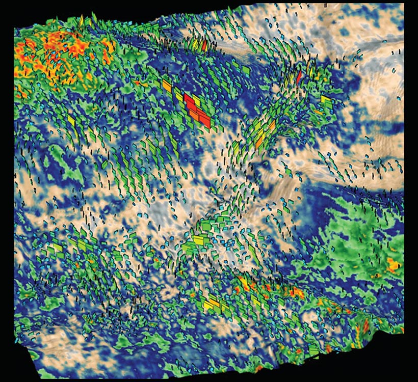
The various azimuthal techniques use different approaches to measure seismic anisotropy. They examine different seismic properties in the light of different bandwidths. When used in combination – and with interpretation guided by realistic rock physics frameworks – these techniques can provide the geophysicist with a comprehensive and thoughtful characterization of fractures in complex reservoirs (Figure 7). While it was beyond the scope of this paper to include examples illustrating these different techniques and showing interpretations, the interested reader will find successful applications in the references. The authors are also available to discuss this further (corresponding author: franck.delbecq@cggveritas.com).

Acknowledgements

The authors would like to thank our many colleagues who generously offered helpful advice and suggestions, Benjamin Roure, Richard Bale and David Gray for giving their time and feedback, and Jan Dewar for her assistance in writing this article and being a voice for those who benefit from math-free descriptions.