Marcellus & Utica Shale PSDM Case Study – Improved Structural Imaging and Rock Properties

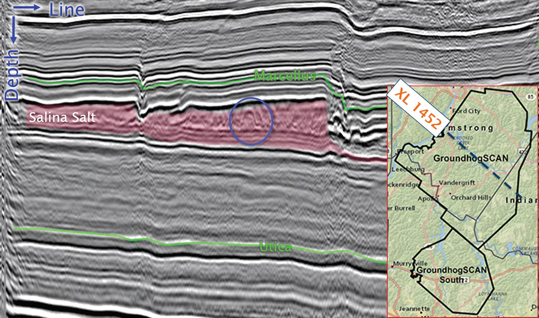
In this abstract, we highlight the performance of PreStack Depth Migration (PSDM) on an ION GeoVentures multi-client survey from northwest Pennsylvania, the GroundhogSCAN 3D. The survey area of interest and a representative crossline are shown in Figure 1. Compressional tectonics during the Appalachian Orogeny shortened the geology above the Silurian-age Salina Salt; here the salt acted as a detachment surface. The overlying Devonian-age Marcellus Shale is heavily faulted and folded, but the underlying Ordovician-age Utica Shale appears relatively undeformed.

First, we show how conventional seismic time processing (PSTM) can increase drilling risk by causing false seismic structures and positioning errors, and by blurring faults and steep dips. We show how PSDM overcomes these hurdles. PSDM can also improve the accuracy of azimuthal velocity anisotropy (HTI) analysis, an indicator of differential horizontal stress (and/or natural fractures), by removing false HTI effects caused by lateral velocity variation. We show evidence that we have detected – only by using PSDM – a vertical change in regional horizontal stress across the Salina Salt.

PSDM Improves Structural Imaging

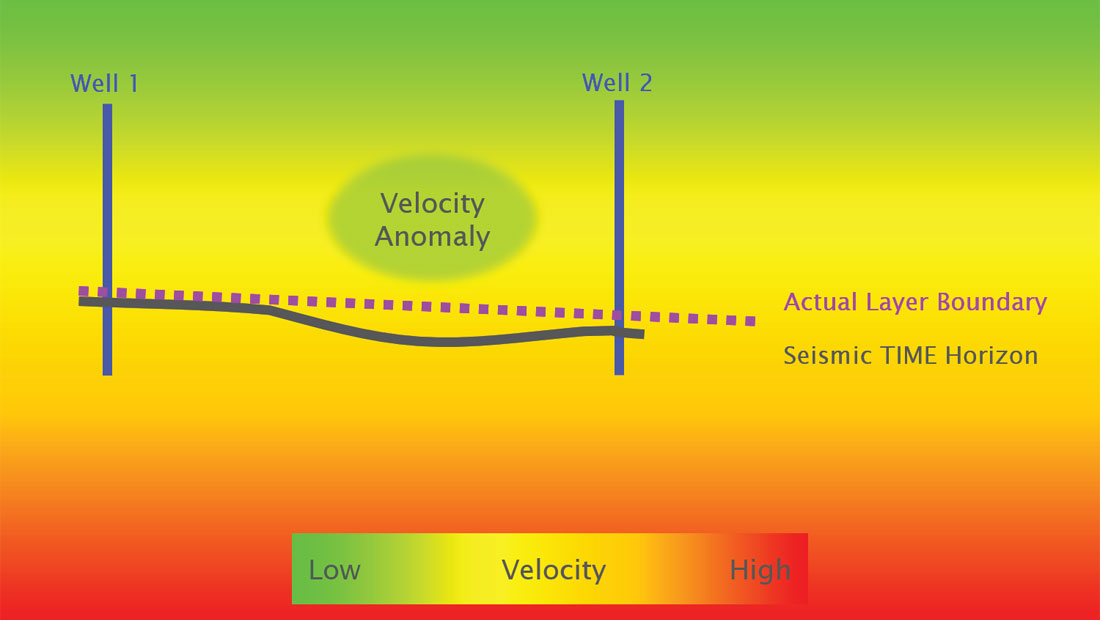
PSDM reduces the risk of dropping out of zone during horizontal drilling. Lateral variations in seismic velocity cause distortions on PSTM images. As Figure 2 shows, if velocity anomalies fit between existing well control, a driller might believe that the time structure represents actual geology. While corrections could be made with LWD data, it’s likely that the confusion caused by the false seismic structure would lead to “porpoising” and reduce the well’s productivity. On the other hand, PSDM can, with an accurate velocity model, remove false seismic structures and help keep the drill bit in zone.

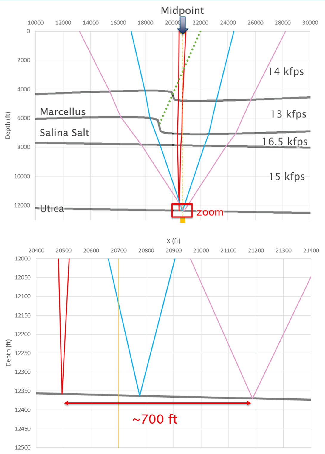
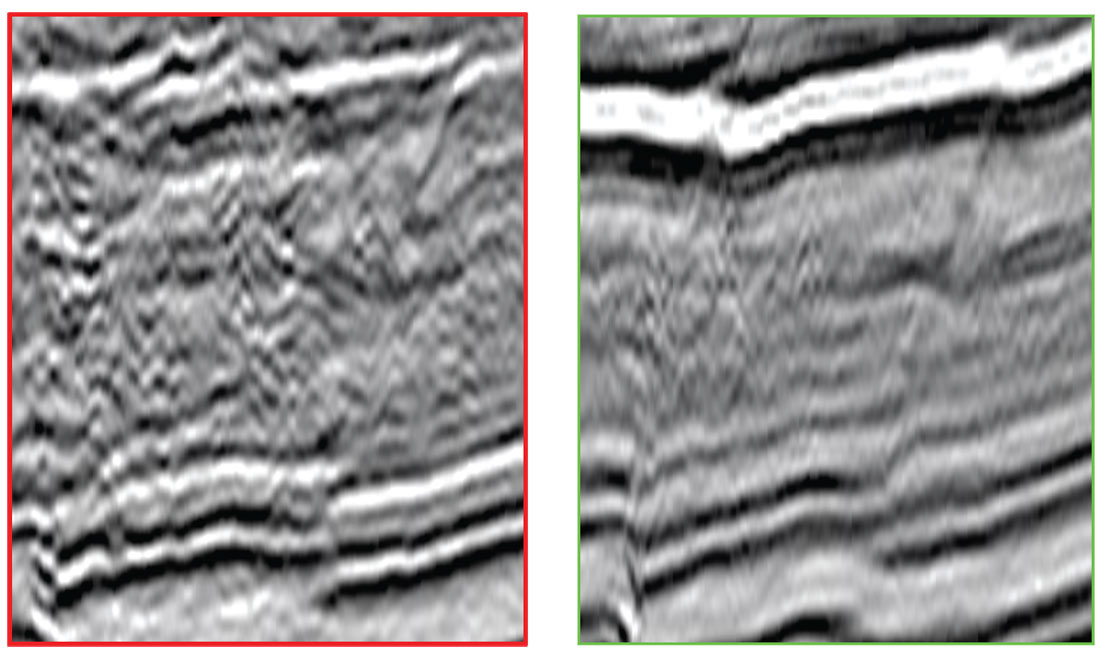
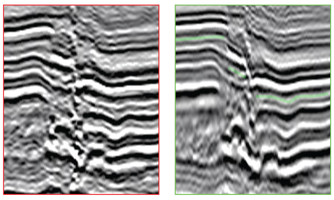
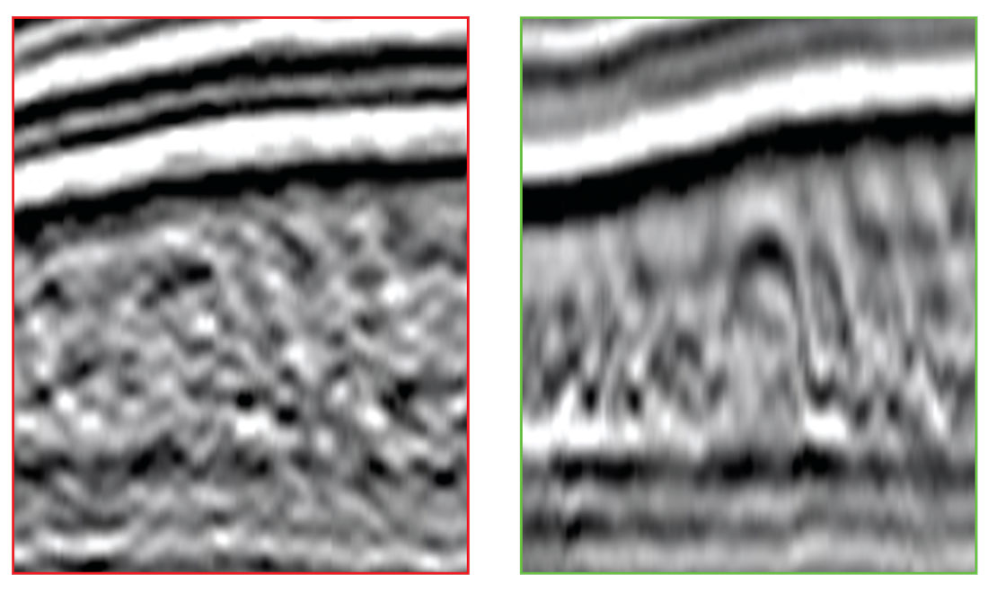
Lateral velocity variation also blurs the imaging of fault planes and steep dips and causes lateral mispositioning of these key features. Figure 2a illustrates how the reflection points for the traces in a common midpoint gather are actually spread over 700 ft. In this case, when we stack the Utica Shale event on a PSTM offset gather, we’re also stacking across 700 ft of midpoint. We stand the risk of smearing steep dips and faults, as Figures 3-5 show. PSDM overcomes this deficiency.

PSDM Improves Azimuthal Anisotropy (HTI) Analysis

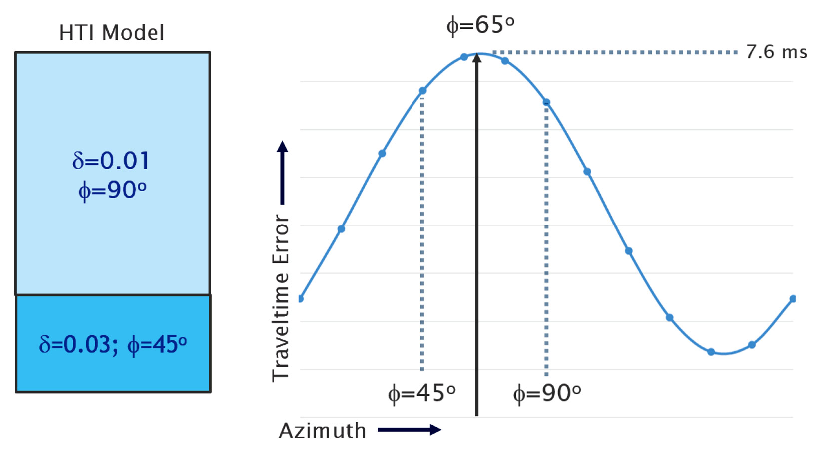
Idealized vertical fractures and/or differential horizontal stress are known to cause seismic velocities to vary as a function of azimuth. This is known as azimuthal anisotropy (HTI). By measuring HTI with seismic data (azimuthal traveltime variations), we can infer the presence and direction of the fractures or differential horizontal stress. This has obvious implications for the optimization of hydraulic fracturing.

In theory, vertically-oriented fractures will produce a sinusoidal traveltime pattern versus azimuth. We typically measure two attributes from OVT (Offset-Vector Tile) gathers – “V_fast-V_slow”, an estimate of the magnitude of the HTI effect, and “V_fast azimuth”, the direction of the fast velocity.

However, lateral velocity variation can cause significant false HTI effects to manifest on OVT PSTM gathers, as Figure 6 below shows. An operator might mis-interpret the false HTI effect as a localized zone of fractures and/or mis-interpret the direction of maximum horizontal stress. Luckily, PSDM correctly handles lateral velocity variations, and can remove false HTI effects from OVT PSDM gathers.

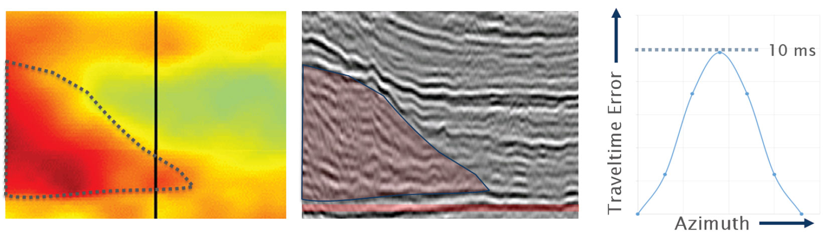
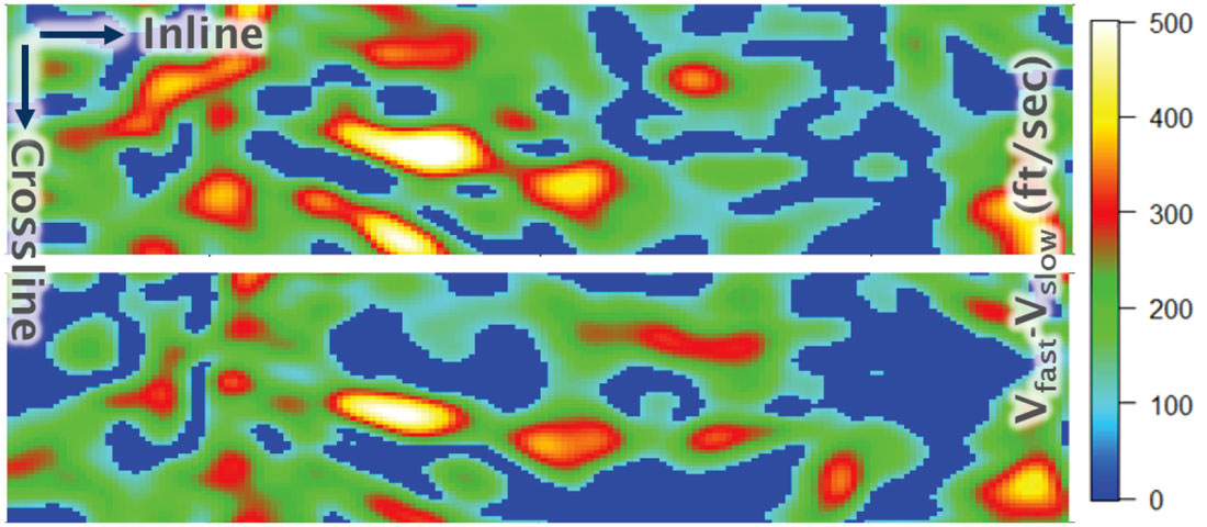
Figure 7 below displays a map, centered on XL 1452, comparing the RMS V_fast-V_slow HTI attributes at the Marcellus Shale, generated by PSTM and PSDM. Although the calculations are made in exactly the same way, the magnitude, on average, is smaller on the PSDM-derived attribute. This indicates that PSDM has likely removed some false HTI effects, leaving behind the true HTI response.

Originally, most HTI analysis didn’t correctly handle vertical variations in HTI orientation – the calculations were “RMS” in nature. The “Generalized Dix Equation” was introduced in 1999 by Grechka et al., and enables us to derive interval HTI attributes, as Figure 8 illustrates.

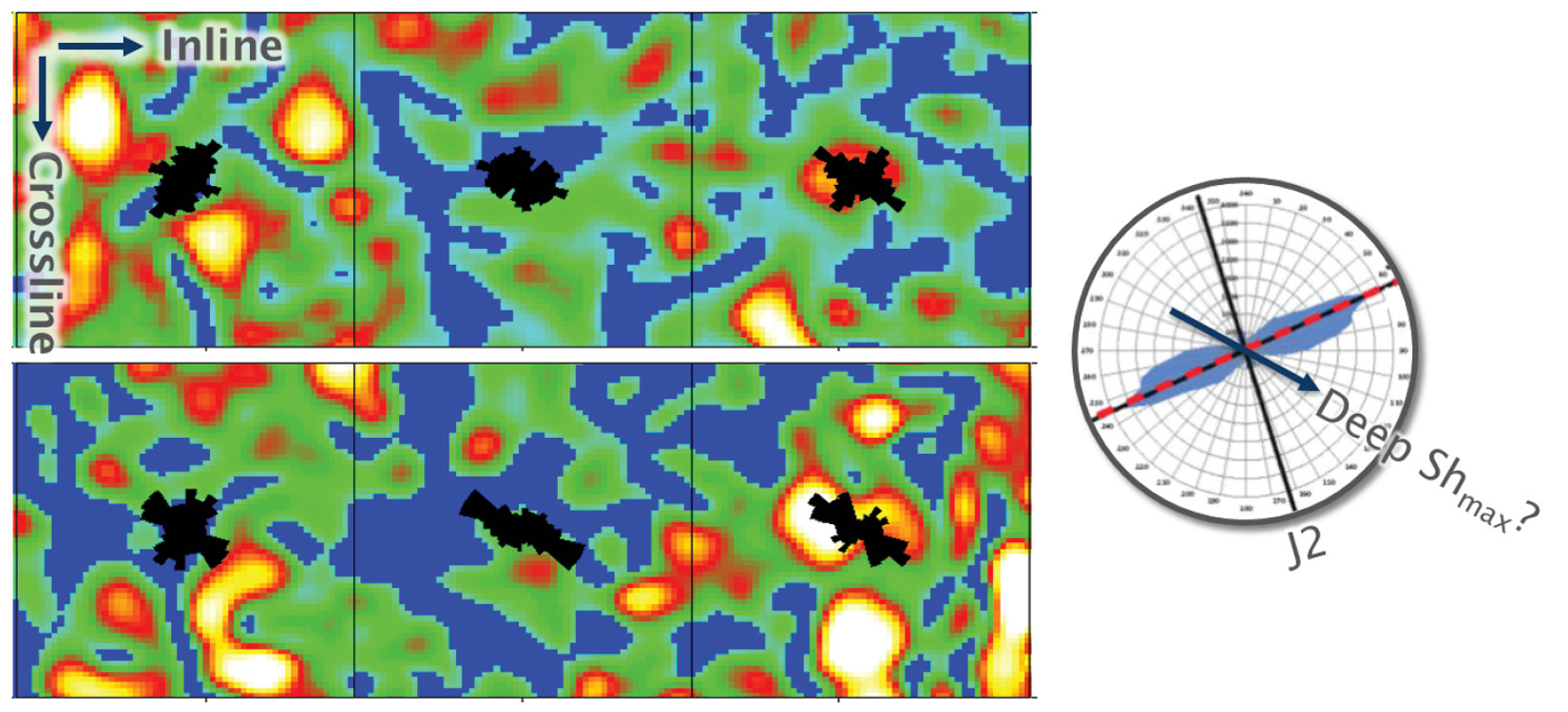
Even when we use interval HTI analysis, the HTI response measured from PSTM will be contaminated by lateral velocity variation. This problem will become acute when we perform HTI analysis on the deep Utica Shale, because of the significant variations in Salina Salt thickness above the Utica. Figure 9 below illustrates interval HTI analysis at the Utica Shale, using both PSTM and PSDM inputs. PSTM provides a muddled view of V_fast azimuth, whereas PSDM provides a far more consistent V_fast azimuth, differs from the shallow V_fast azimuth.

Interpretation

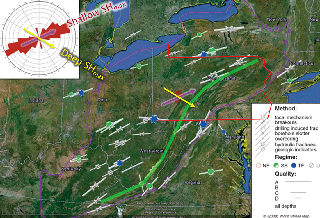
Figure 10 compares the V_fast azimuth direction computed at the Marcellus (green) and at the Utica (blue). In general, V_fast azimuth is believed to align with present-day SHmax. V_fast azimuth from the surface to the Marcellus is, interestingly, perpendicular to the direction of compression. The green arrow aligns with the SH_max from the World Stress Map. Although the Appalachian Orogeny no doubt caused compression of the shallow section, if the shallow section was currently under compressive stress, we’d expect shallow SH_max to be parallel to the compression; instead, it is roughly perpendicular. Intriguingly, the deep V_fast azimuth direction that we measured at the Utica is aligned with the direction of paleo compression.

Conclusions

We demonstrated that PSDM has significant utility in the Western Pennsylvania Shale Basin, although the technology has not (to date) been frequently utilized. PSTM appears to yield a “good image” in most areas, but there are subtle-but-crucial differences in the structural image quality (faults and steep dips), caused by lateral velocity variations. Additionally, PSDM appears to “simplify” local structures around the Marcellus Shale that are horizontal drilling targets.

Secondly, we demonstrated how PSDM provided a superior input for HTI analysis. By removing false HTI effects from OVT gathers, PSDM produces more reliable azimuthal attributes. Intriguingly, by utilizing interval PSDM HTI analysis at the Utica Shale, we detected a consistent V_fast azimuth direction (not interpretable on the PSTM attributes) which differed from the shallow V_fast azimuth. From available well data, we observe a change in the differential stress across the salt, so it is reasonable to see a stress rotation as well. For what it is worth, the measured deep V_fast azimuth is perpendicular to the trace of the Appalachian Mountains, and presumably parallel to the paleo SHmax direction.

Acknowledgements

We thank the management of NEOS for permission to publish, and to ION Geophysical for the right to show the data examples. We also thank for their valuable feedback many colleagues at NEOS, as well as countless attendees of geophysical luncheons where this work has been previously presented.