Processing Considerations for 3D VSP

Abstract

VSP surveys have long been known to produce superior reflection images compared to images from surface seismic. The literature is rife with examples showing the advantages of the VSP method. This paper shows how 2D and 3D VSP data is processed with practical state-of-the-art technology and algorithms. The key steps in the processing flow are described and illustrated with figures. The flow presented defines a practical method of processing VSPs, which has been successfully employed in commercial VSP processing. As with surface seismic processing, alternative methods do exist.

We would like to thank the EAGE for permission to reprint this article. The original paper was previously presented in the EAGE First Break Volume 26, July 2008 under special topics, Well Technologies.

Companies today have a need to better understand and monitor the production from their existing reservoirs. With the proliferation of large borehole geophone arrays, 3D VSP has become a viable option for monitoring what’s happening around a well. With geophones fixed in the borehole below the surface, increased resolution at the reservoir level is possible. In this article we will look at the processing of a 3D VSP volume and some of the complexities involved.

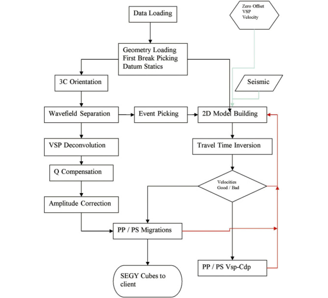
In Figure 1 and 2 we compare the processing flow of a typical 2D walkaway VSP with that of a 3D VSP. Note the similarity of the two flows. In actuality they are almost identical, except that one is 2D and the other 3D.

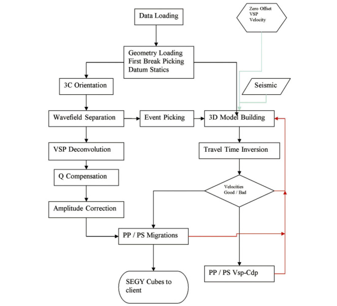
The major differences between 2D and 3D are in the increased dimensions of the velocity model, the 3D migration and in the volume of data. 3D VSP data typically contain many times the amount of data as a walkaway survey. This volume of data creates challenges at each step in the processing.

Geometry and first break picking

As with any seismic survey the recorded data must be mapped to the survey position data. Before a survey can be processed, the geometry must be loaded to the data headers and verified. The QC of the 3D VSP geometry involves observing first breaks and 3C rotation angles with respect to shot-receiver positions.

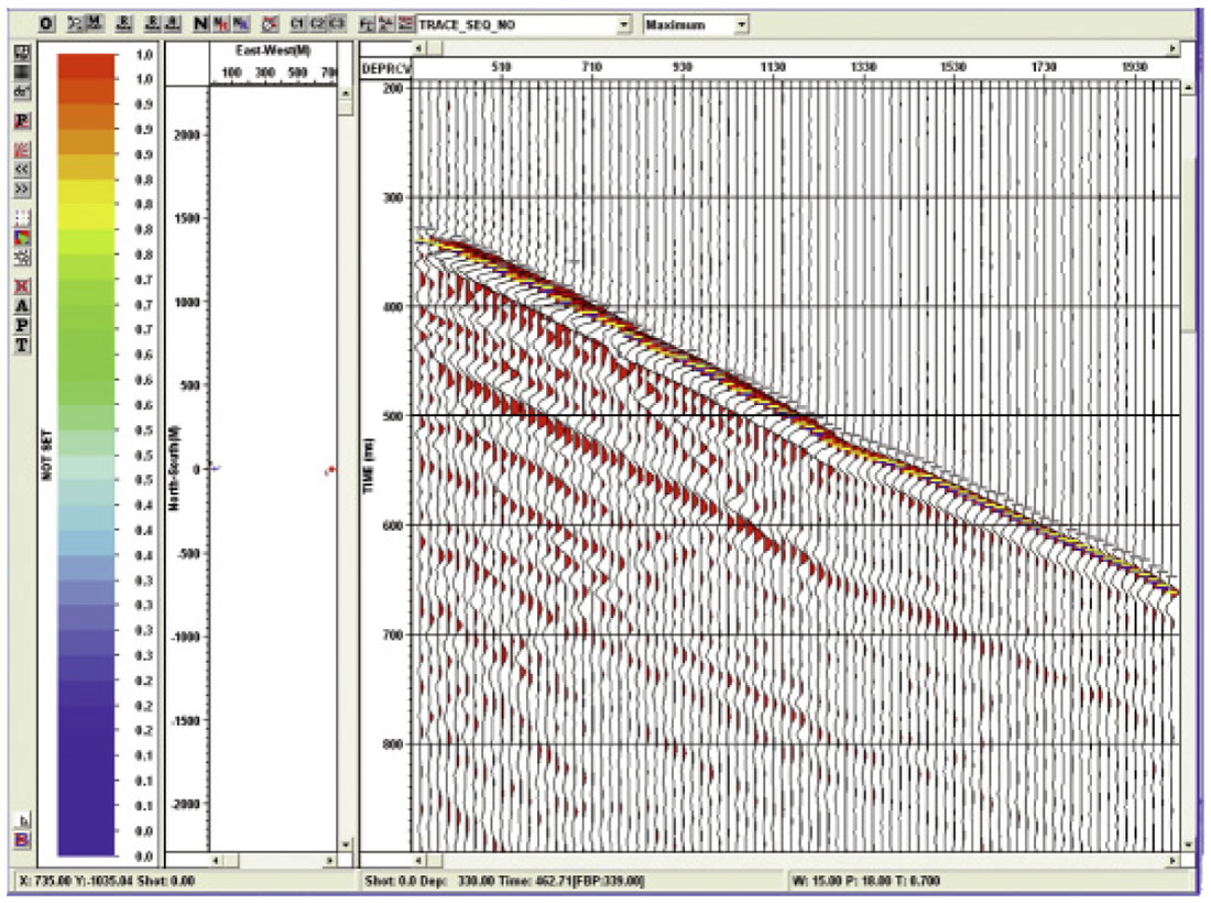
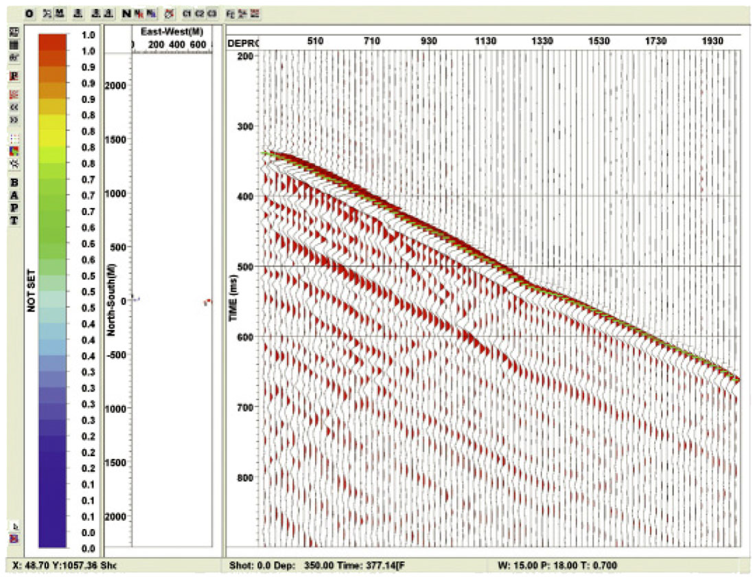
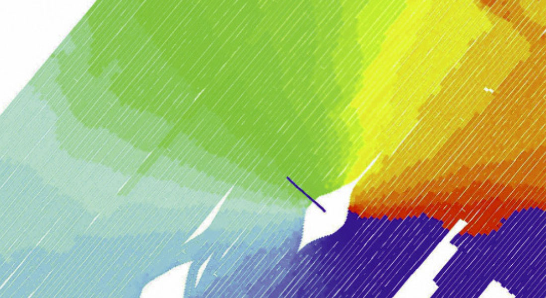
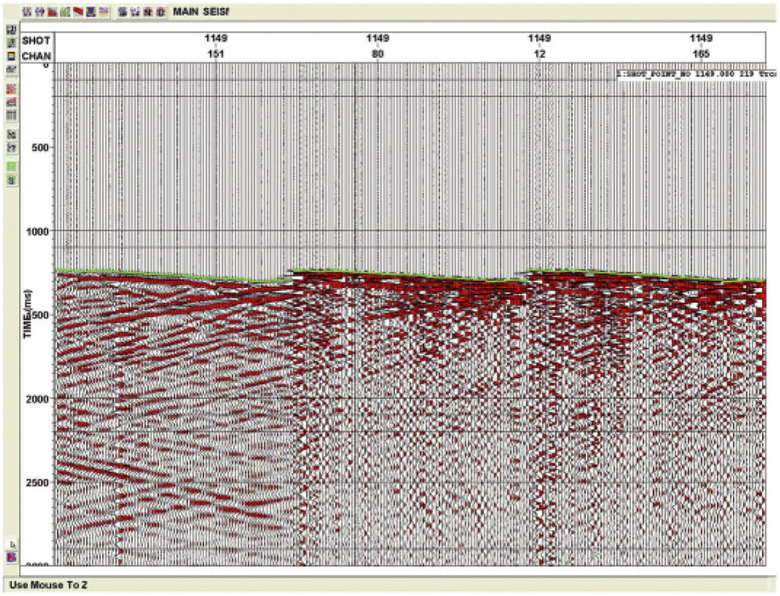
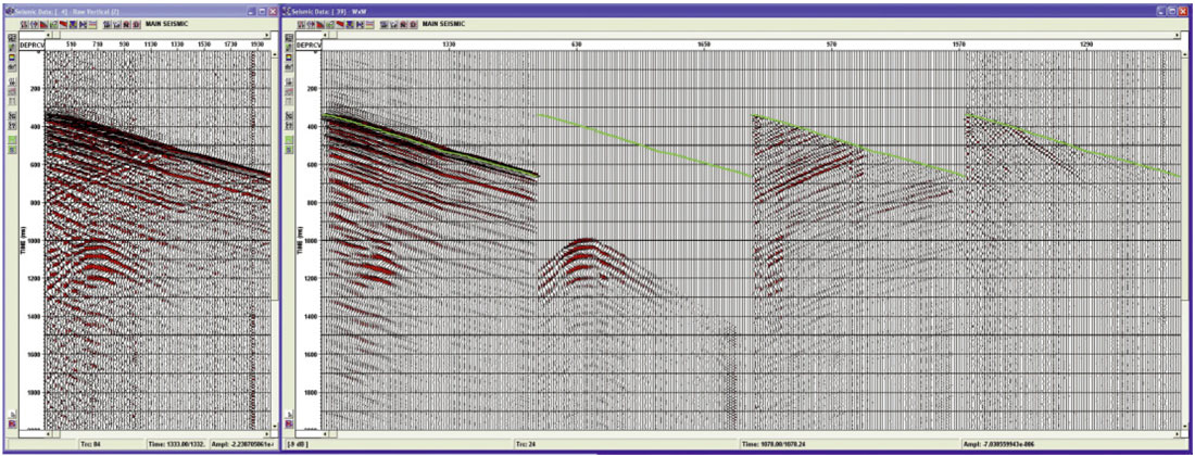
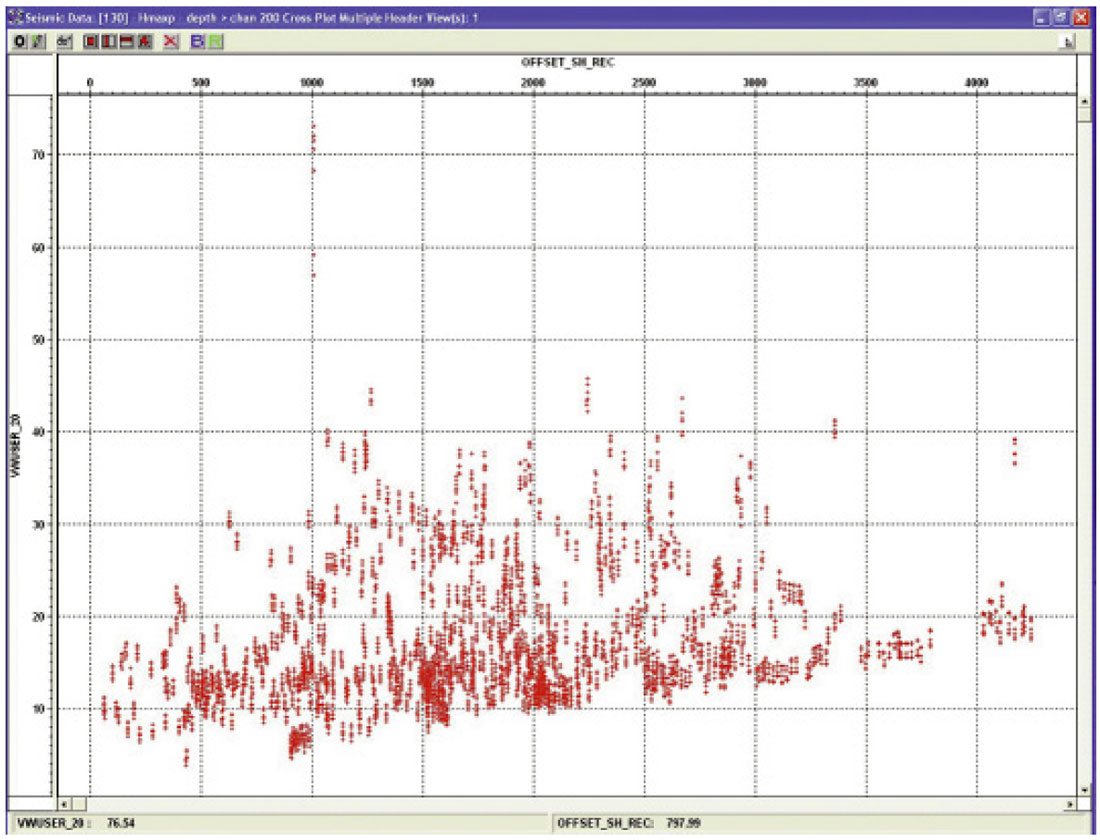
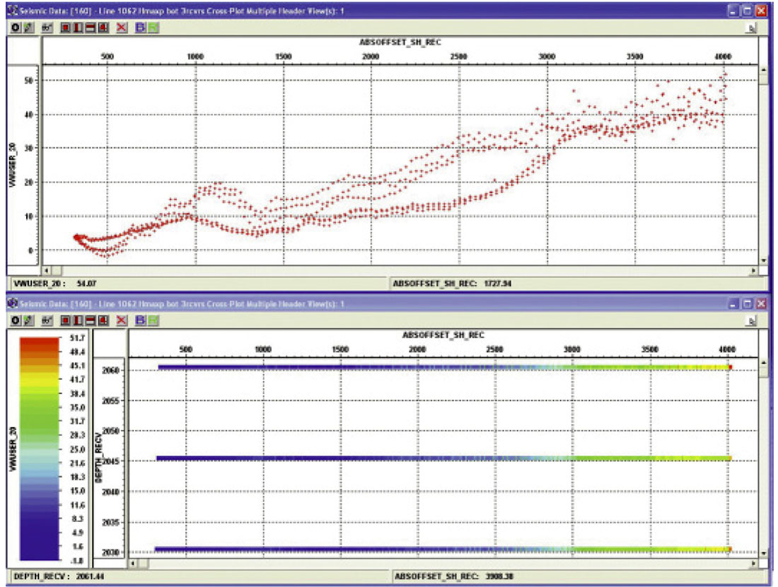
After, or concurrent with, the geometry loading, the first breaks are picked. This picking can be a very involved process for 3D VSP. Imagine a single offset VSP takes 1 minute to pick the breaks manually. Then for a marine 3D VSP with 30,000 shots this process would take 30,000 minutes or 500 man hours (62 man days of work). Obviously an automatic picking method is required to speed this process up. Figure 3 shows automatic first break picking based on 3 different criteria. These include Largest Amplitude (blue), Polarization (yellow) and Amplitude threshold (grey). Figure 4 shows these same picks with the final picks in green that are derived from the automatic picks based on an initial seed pick.

In marine applications picking the first arrival is usually straightforward because the source energy level remains constant, as does the medium surrounding the source. In addition the shot elevation remains relatively constant, and the geometry is such that offsets away from the wellbore usually increase in an even progressive manner. In land, shot to shot variations along with elevation changes can make automatic picking of VSP data extremely difficult. If elevation changes are extreme, a datum static should be applied before first break picking to better align the shot to shot differences.

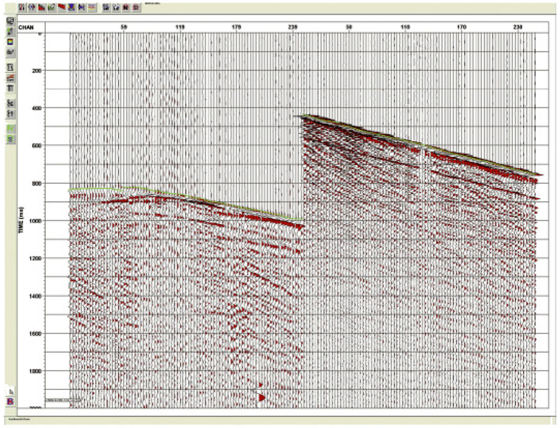
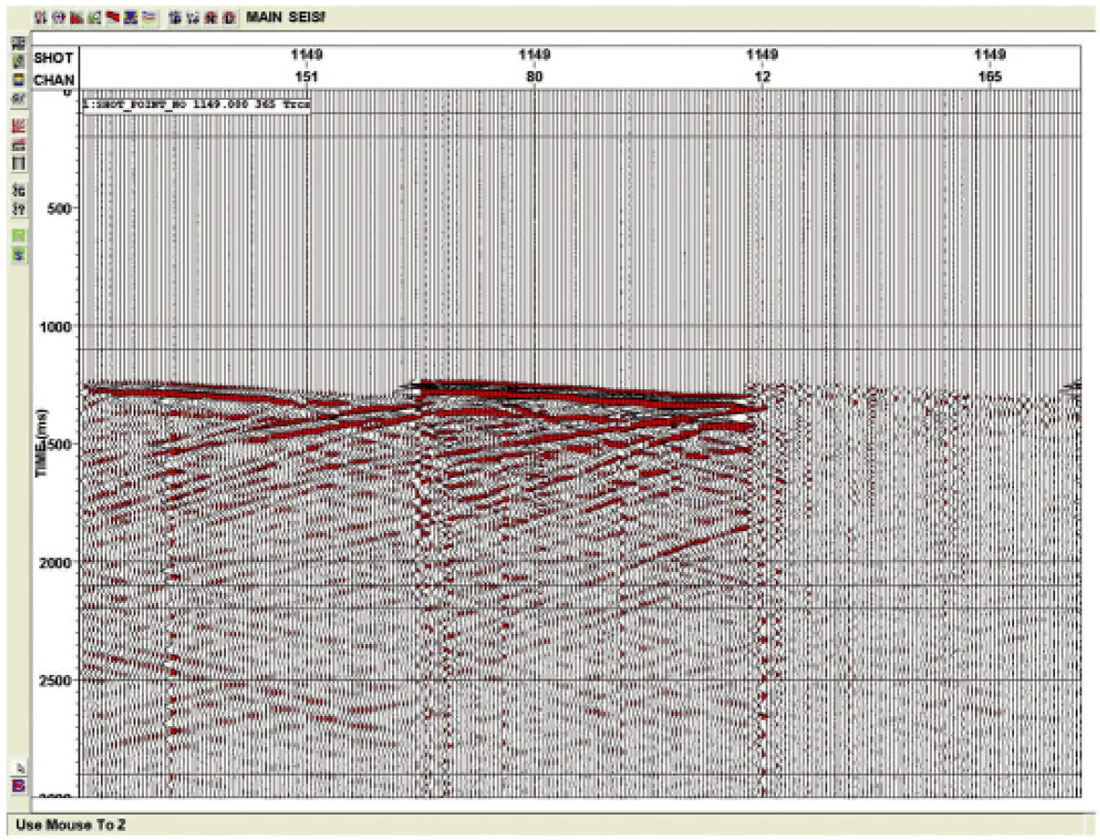
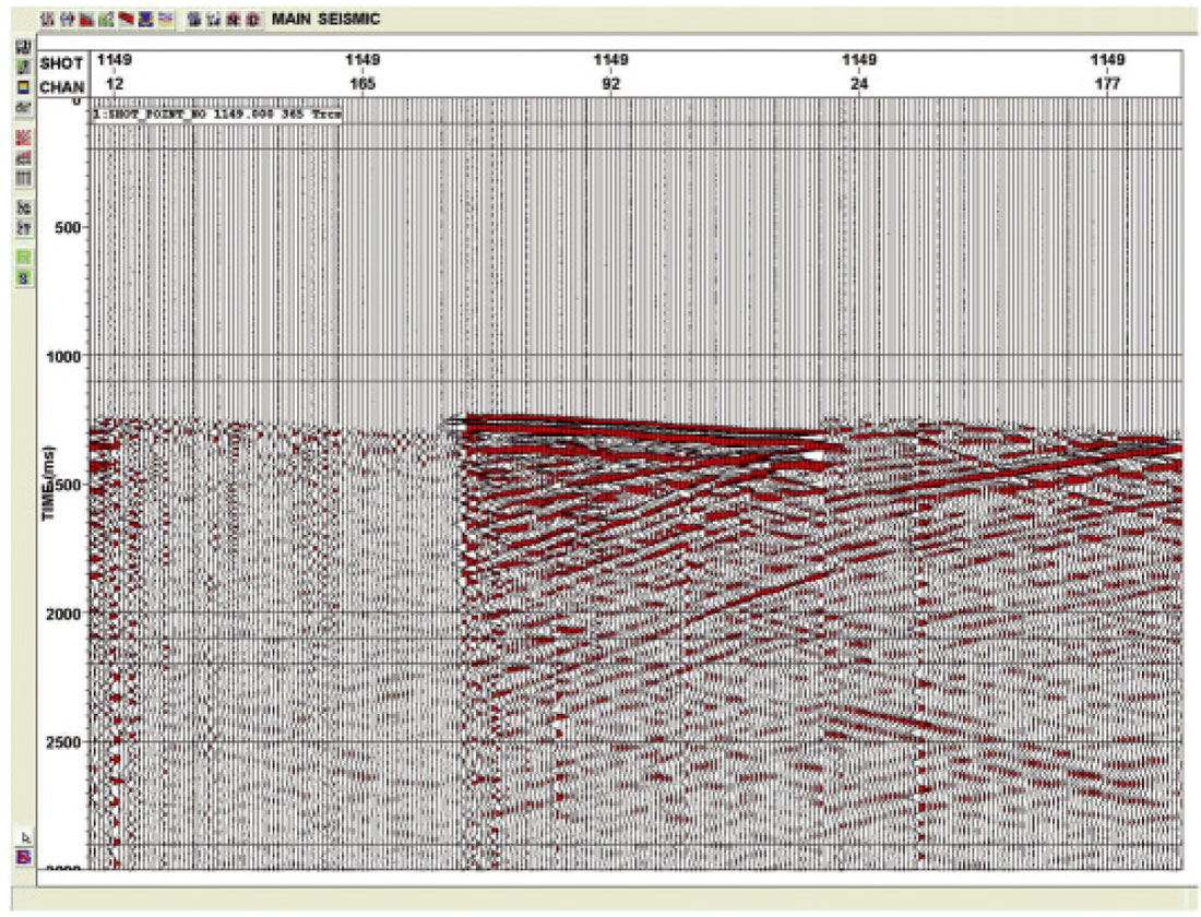
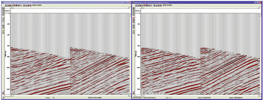
In addition to picking problems caused by statics, another pitfall arises as the receiver levels get shallower and offsets get longer. The first arrivals become refractions instead of down-going direct arrivals, leading to a polarity reversal on the vertical (Z) channel. Most manual picking is done on this vertical channel thus the first break picks often jump a half cycle above the refractor depth. This is shown in Figure 5. On the left is a long offset and on the right a near offset. The first arrivals are shown in green.

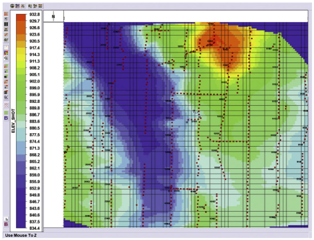
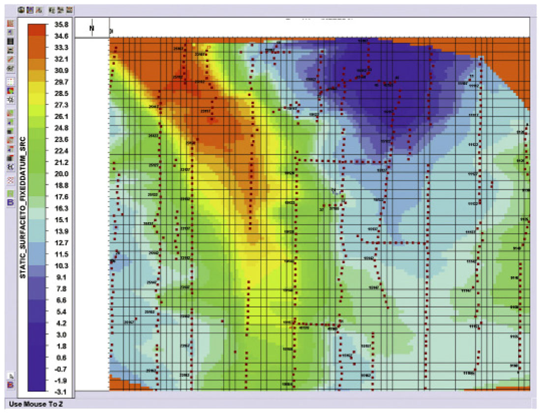
In Figure 6 we see the elevation across a VSP survey. Figure 7 shows the datum statics computed and Figure 8 shows a receiver gather after and before application of the datum statics. Note the improvement in the continuity of events on the left after datum statics are applied. The first breaks in green also show much less variation as they increase in time as offset increases from left to right.

After completion of the first arrival picking, first break picks for individual receiver gathers should be viewed to note any anomalous picks. In Figure 9 the first arrivals are mapped (0 ms is dark blue). Travel time from shot to receiver increases proportionately with offset away from the central receiver.

3C Orientation

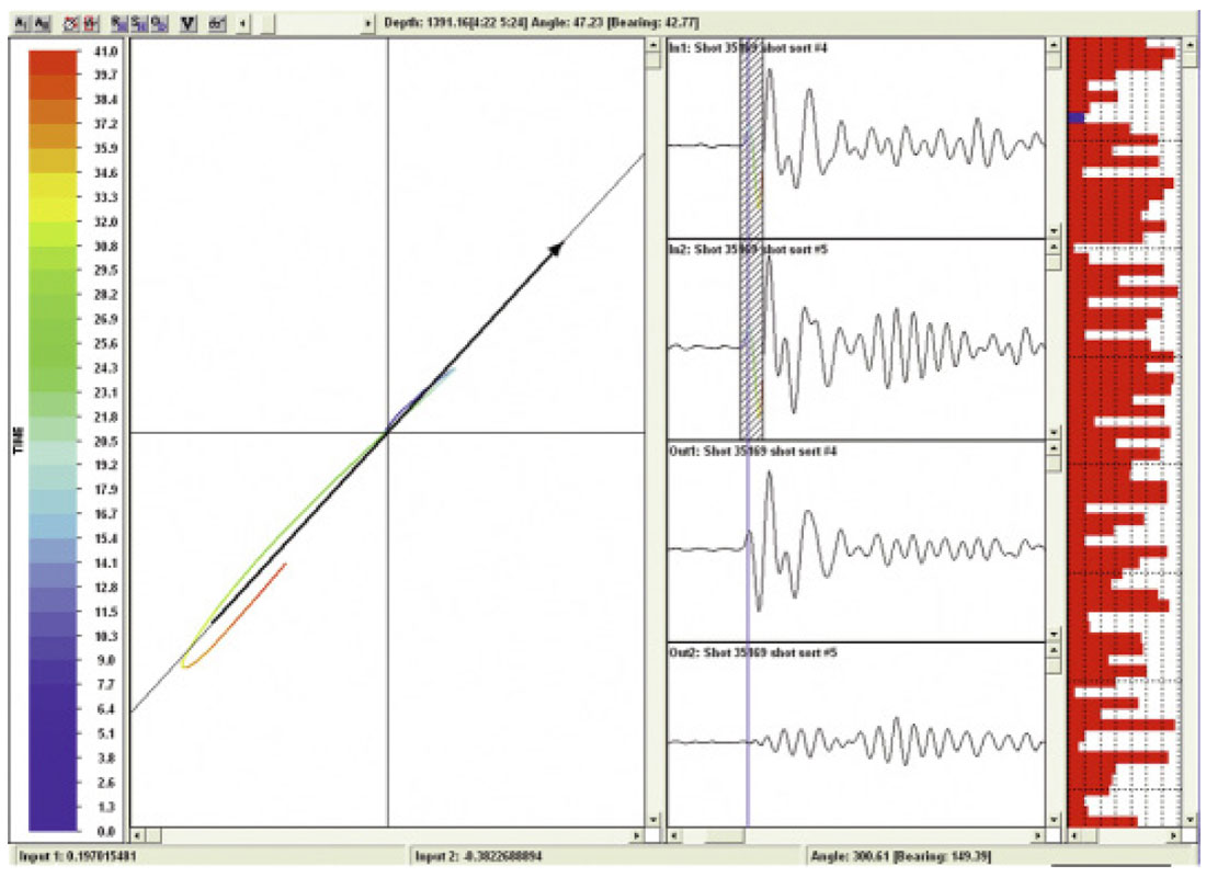
The 3C data is first rotated in the horizontal plane to orient one component inline with the source-receiver direction (often referred to as the horizontal radial component or Hmax) and the other component orthogonal to this (transverse component or Hmin). The transverse component captures the SH (horizontally polarized shear) wave-field as well as out-of-plane reflections. The radial component (Hmax), along with the “vertical” component, captures the remaining wave-field consisting of downgoing P and SV and up-going P and SV waves. Figure 10 shows a hodogram of the two horizontal components. Amplitudes in a time window bracketing the first arrival of the X and Y traces, shown in the top 2 trace panels, are plotted on the X and Y axes of the hodogram. A linear least squares fit line determines the computed angle of orientation. The angle is applied to the data (bottom 2 trace panels) through a rotation matrix. Note the rectilinear nature (the hodogram is almost a straight line) of the data displayed in the hodogram. This is a good QC of the noise and coupling of the geophones. On the far right are the computed angles for all levels of a single shot. The randomness of the angles results from the tools being cabled and un-oriented in X and Y with respect to one another in the borehole.

With 3D VSP the number of shots makes it prohibitive to do the rotations manually. For vertical non-deviated wells a method can be employed whereby only a few shots around the wellbore are rotated. Knowing the source-receiver azimuth, the orientations of the horizontal geophones are determined for each of these selected shots and an average is taken. The remaining shots are rotated based on the difference between the source-receiver azimuth and the estimated X,Y geophone azimuth. This method assumes that the raypaths from source to receiver are linear and direct. Another method uses principal components of the eigenvalues over the first arrivals, and is computed for all shots. Figure 11 shows the rotation angles of a single receiver gather for all shots after automatic rotation. The radiation pattern of the computed angles is nearly linear away from the well bore (0 degrees is dark blue proceeding clockwise around to 360 degrees in red). This shows that the averaging method above would work well in this case with minimal error in the computed angle. The automatic method is a useful tool for shot location QC. In land 3D VSP shots are mapped to a FFID in an observers report. This assumes that the shooter or vibrator operator were actually at the shot specified especially when no GPS verification is used. The hodogram can show within a few degrees if a shot was actually misplaced azimuthally but the correct offset cannot be shown. QC of the first breaks can help in regard to this.

Rotation for All shots

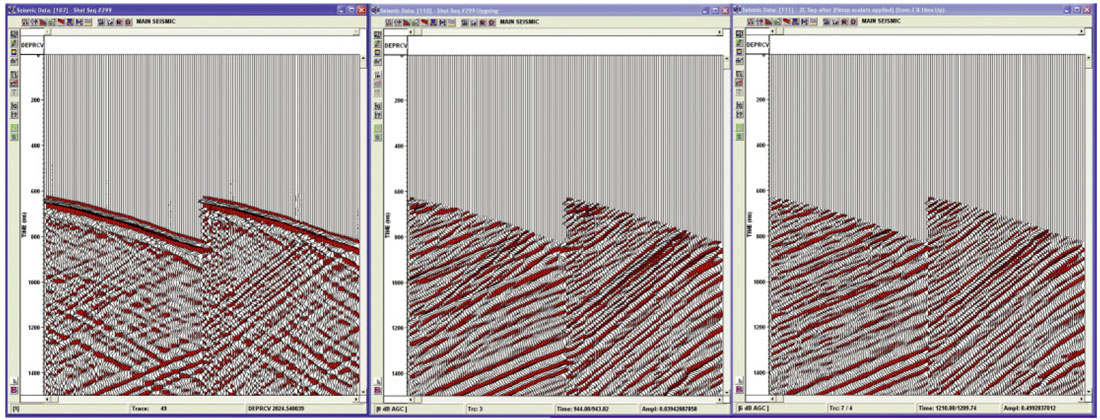
Figure 12 shows Z, X and Y components of a VSP shot record. The first rotation is performed on the X and Y components to orient one geophone in the direction of the source (Hmax) and the transverse component (Hmin). The data shown in Figure 13 shows Hmax and Hmin components after the first rotation. There is little energy except noise remaining on the Hmin channel indicating there is minimal SH energy or out of plane reflections. Figure 14 shows the results of the second rotation for the same shot record. Input is the Z and Hmax components in figure 13. Output is Hmin, Oriented and Transverse components. The Oriented component is aligned toward the source and contains all the down-going P wave energy. The Transverse component now contains the down-going SV data.

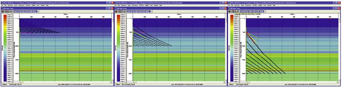
The two rotations shown in the previous figures have a single angle for each receiver source pair effectively isolating the downgoing P and SV wave-fields from each other. The up-going P and SV wave-fields still exist, mixed on both channels. This results from differing angles of incidence of reflections with depth as well as the difference in reflection angle between the P and converted SV waves. After the down-going wave-fields are separated, the remaining up-going wave-fields need to be rotated onto separate components in a time-variant manner to capture all the energy for each up-going wave-field (P or SV) This can be accomplished using a model and calculating the angle of incidence of P and SV waves at all time points on the VSP data. Figure 15 depicts a velocity model in depth and the calculation of angles into geophones from key reflectors at varying depths. Note the change in angle of the ray arriving into the geophone as the reflecting events get deeper, shown with red, green and yellow arrows. Another method for computing these arrival angles is the plane-wave decomposition approach in either the FK or tau-p domains. In these methods the data is separated as a function of vertical slowness and P and SV wave velocities. Figure 16 shows the Z and Hmax up-going components on the left, and the P and SV separated data after time-variant rotation on the right. Figure 17 shows the Z and Hmax components on the left, the Z and Hmax components after down-going separation in the center, and the separation of the P and SV wave-fields based on plane wave decomposition in FK space on the right.

Wave-field Separation

Following or in conjunction with the 3C orientation (as shown previously) the wave-fields are separated. Many methods have been employed to separate wave-fields such as FK, Median, Tau-P, as well as Parametric and Waveby- Wave. Each method can work well depending on the VSP data set.

In Figure 18 the down-going P, shear headwave, and up-going P wave-fields were isolated onto separate components. These were separated using a Wave-by-Wave approach. The downgoing P wave can be used in deconvolution, although for walkaway and 3D VSP this is often not the case. The downgoing wave-fields yield velocity and attenuation information that can be applied to the processing of the separated up-going wave-fields.

VSP Deconvolution

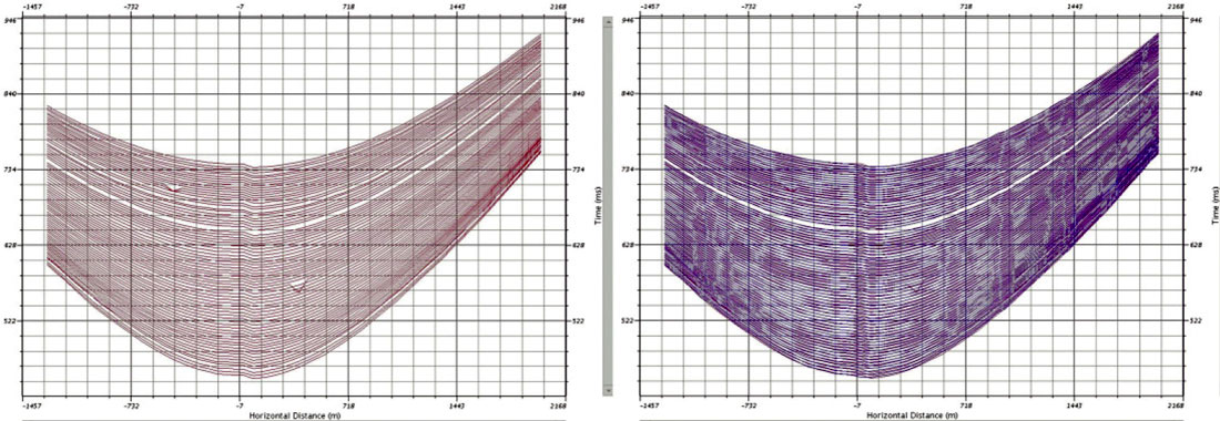
In VSP the geophones are placed beneath the surface of the earth and measure the down-going injected wavefield as well as the reflected up-going wave-field. It is common to use the down-going P wave (the measured wavelet) to design an operator to deconvolve the VSP up-going or entire wavefield. This works well for near offset VSPs but as the offset increases, the ray paths of the down-going and up-going wave-fields are no longer coincident and the criteria for using the down-going as the decon operator (ie. the assumption of consistent multiple reflection train character) breaks down. This usually occurs on the medium to long offsets of walkaway and 3D VSPs where maximum offsets equal the depth of the target. The down-going and up-going wave-fields must first be separated and then, like surface seismic, predictive deconvolution can be used to aid in removing longer period multiples. This is followed by spiking or surface consistent deconvolution to whiten and convert the data to zero phase. A near offset shot can be isolated and a standard inverse-operator VSP deconvolution applied. This deconvolved shot is then compared to the final phase of the 2D or 3D volume and the data volume is adjusted. In Figure 19, VSP inverse operator deconvolution is applied to the down-going wave-field on the left. The first arrivals are aligned at 100 ms. On the right, the deconvolution operator (as designed on the down-going) is applied to the up-going wave-field.

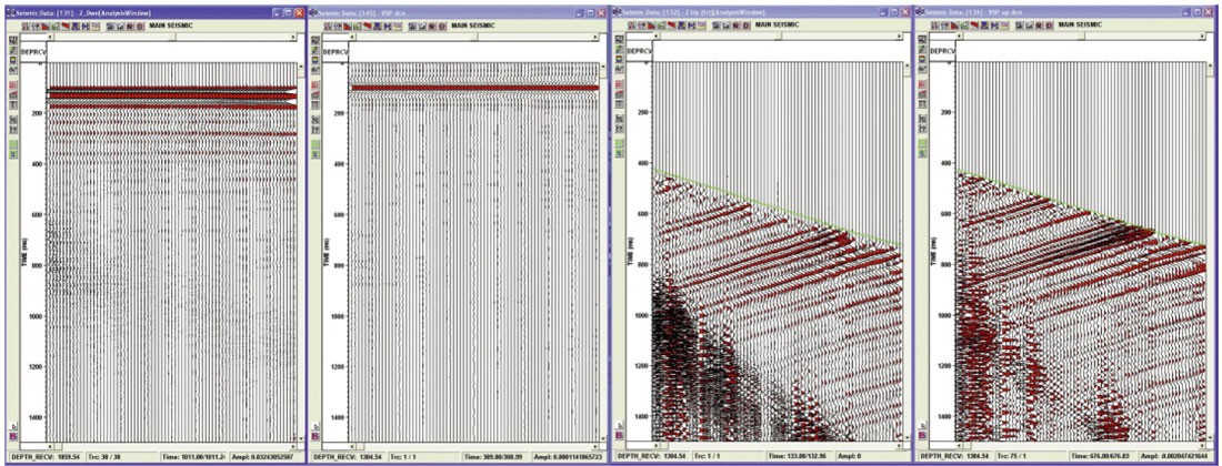
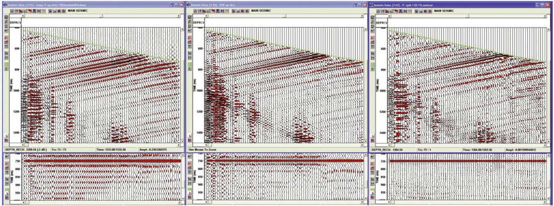
Figure 20 shows a comparison of the VSP deconvolution (center) with the spiking deconvolution (right). The raw data before deconvolution is shown on the left. Autocorrelations for each data set are shown below each panel.

Q Compensation

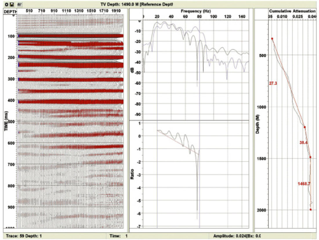
Q attenuation can be calculated using the down-going wave-field of a near offset shot. The VSP down-going wave-field has a high signal to noise ratio and is fairly stable. Hence, the spectral ratio method works well. If the Q attenuation is large, inverse Q filters can be applied to the VSP data following deconvolution. Figure 21 shows the use of the spectral ratio method to compute the cumulative attenuation with depth from the VSP down-going. Q is computed over constant attenuation intervals.

Amplitude Correction

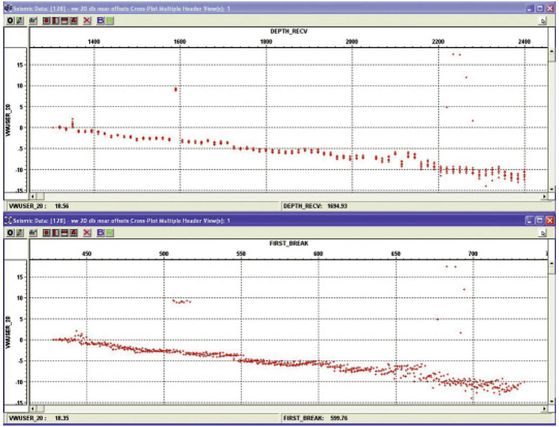
After estimation of Q, amplitude corrections must be applied to compensate for spreading loss, coupling and shot to shot variations. These can be applied individually or in a shot consistent manner. Figures 22a, 22b, and 23 illustrate how the first arrival energy of the oriented data is used to determine attenuation as a function of depth, time and offset. Variations from the trends are a result of geophone coupling or shot to shot amplitude differences.

Velocity Model Building

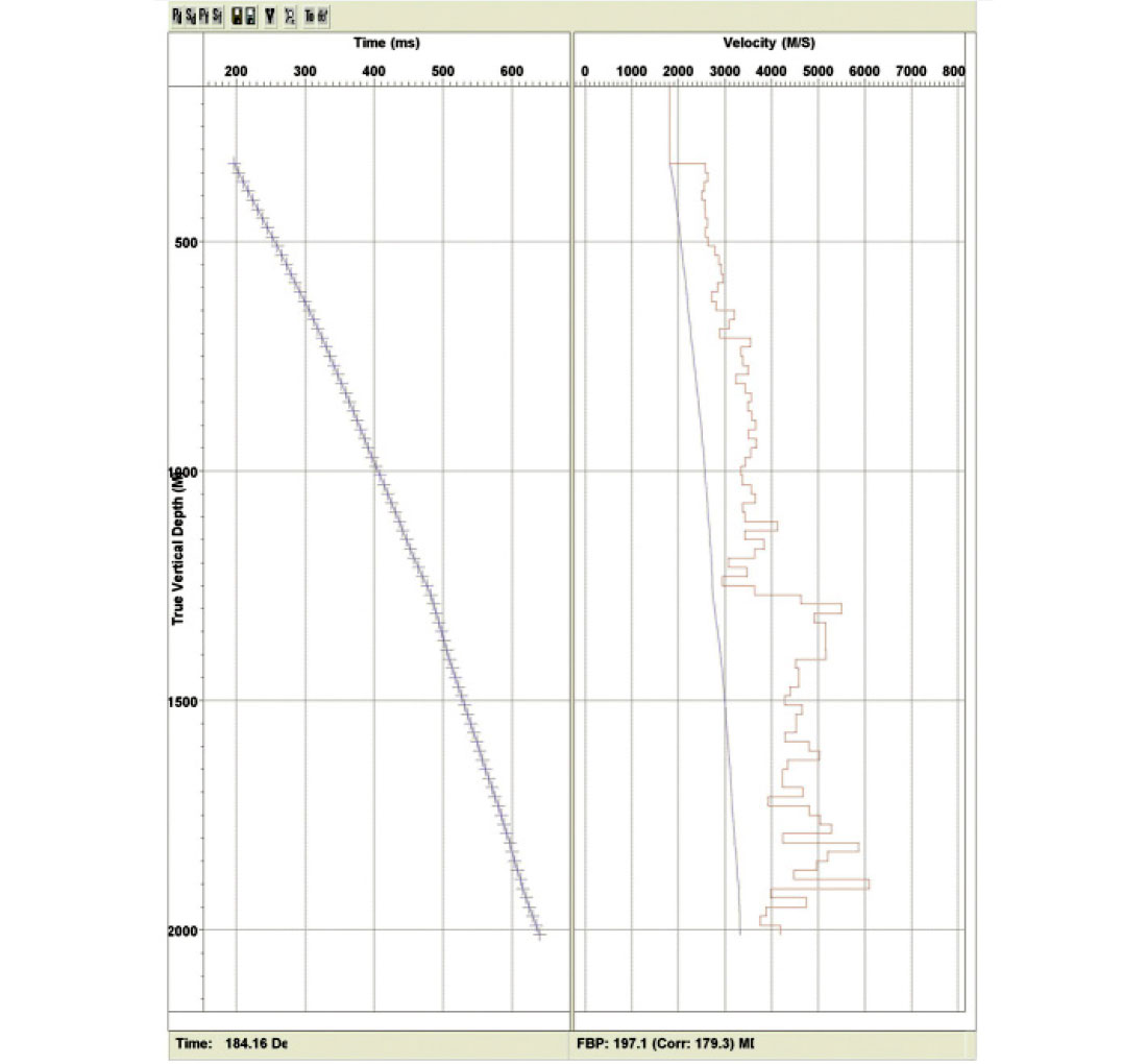
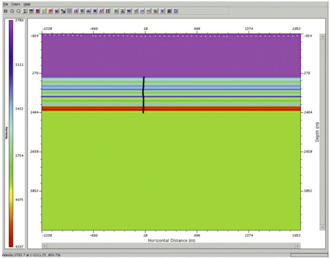
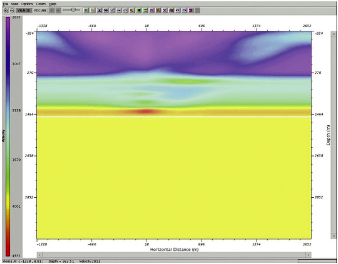
To obtain the velocity model, a 1D near offset velocity function is extrapolated into 2D or 3D space. Usually the model begins as a flat layer model. Layer dips or structure can be adjusted as determined from surface seismic. Figure 24 shows the near-offset velocity profile derived from first break times. Figure 25 shows a subsequent extrapolated 2D velocity model.

Tomographic Inversion

The initial velocity model is ray traced and the modeled arrivals are compared to the actual first break picks. The model is updated until the differences in arrival times from sources to receivers between model and VSP data are minimized. If the inversion does not converge as a result of short wavelength statics, residual statics are applied and the inversion is run again. Figure 26 shows the comparison between actual and raytraced derived first break times for a 3D VSP. Figure 27 shows a profile through the resulting updated velocity model.

Migration

With the amplitude corrected deconvolved data and the velocity model completed, we can proceed to migration (2D or 3D as appropriate). VSPs are recorded with geophones in the well bore at known depths. Thus VSP migration is normally depth migration. The most common algorithms used are Kirchhoff, Reversetime, and Wave-equation migration. For large volumes of data, Reverse-time tends to be slow and wave-equation migration requires evenly spaced input. Thus Kirchhoff depth migration is used most often. A quicker method than migration is to perform a partial migration process called VSPCDP transformation. This method uses raytracing within the velocity model to place VSP events at their appropriate depth and spatial position. The VSPCDP method can be used to quickly fine tune the velocities of the VSP model before a final migration is performed. CDP depth gathers are created for each receiver level (i.e. a VSPCDP transform is performed for each receiver level). Events in the gathers will have residual moveout, if the velocity model is incorrect.

Figure 28 shows the results of a VSPCDP transform for a 2D walkaway line.

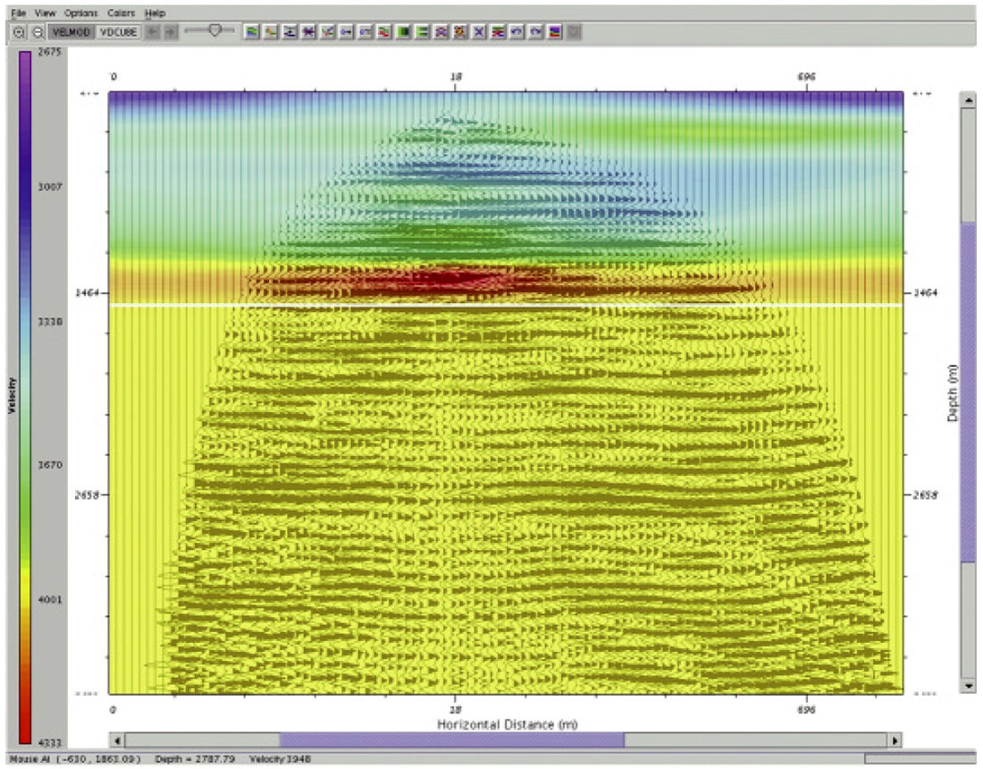
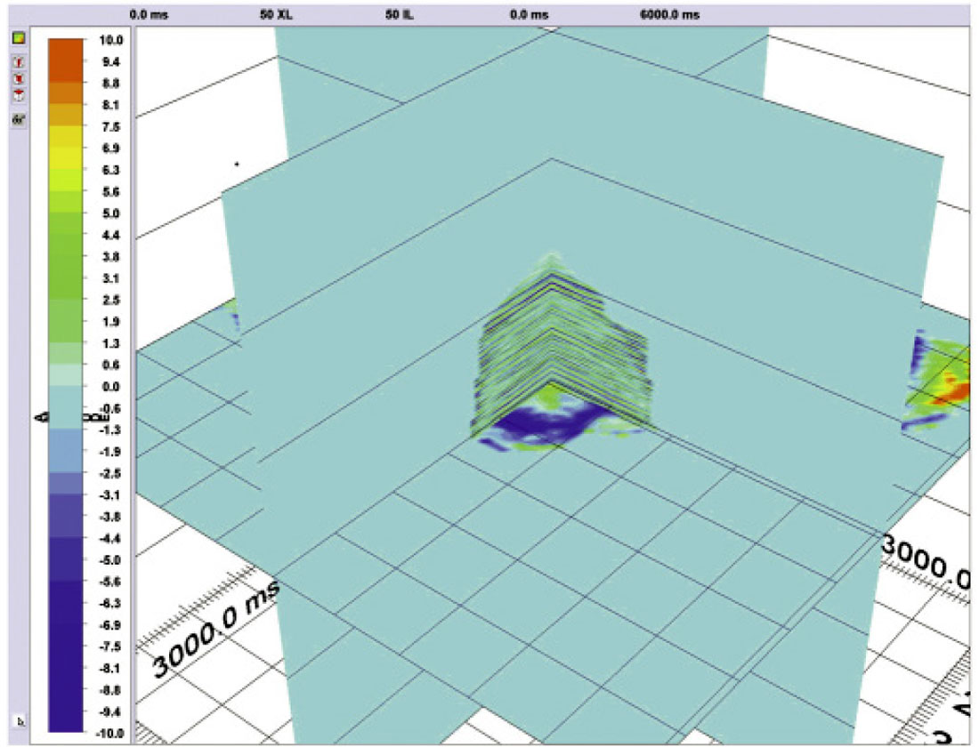
Figure 29 shows a 3D perspective of a 3D VSP volume after Kirchhoff depth migration.

Conclusions

The increased resolution and higher frequency content of the VSP over standard surface seismic makes it an excellent tool both for exploration and exploitation. The advantages of VSP over surface seismic for imaging the structure and stratigraphy around the host wellbore are many. The lateral extent of imaging for a single well 2D walkaway or 3D VSP is significant around the well bore. Assuming that receivers are deployed all the way to surface, the maximum coverage away from the well is about one half the depth to target (e.g. for a 2000m target the coverage has a radius of over 1000m around the well bore). Since the character of the down-going wave-field is actually measured and recorded by the geophones in the borehole, as shown above, the deconvolution of the seismic signal can be approached from a more deterministic perspective rather than purely statistical. This means that the resulting deconvolved seismic image can more closely represent true zero-phase data as compared to deconvolved surface seismic data, which usually has to be checked by a VSP. The quiet wellbore environment, when combined with good receiver coupling, can result in significantly broader band-widths of the final migrated 2D or 3D VSP data as compared to surface 3D seismic. This can dramatically improve both vertical and lateral resolution at the target level. 2D and 3D VSP also provides us with information on the converted Shear wave-field. Thus, in some cases, VSP can provide S/N ratios high enough to facilitate identification and mapping of porefluids and fluid contacts, and thereby facilitate 4D monitoring of target reservoirs.

A processing method for 2D Walkaway and 3D VSPs has been presented. The method is simple and since many of the processes are automated, quick turnaround of the final processed image is possible. This lends itself to being a useful tool in making quick decisions of where to steer the host well while drilling and in determining subsequent drilling locations for reservoir exploitation and monitoring reservoir changes.