Processing 3-C Heavy Oil Data for Shallow Shear-wave Splitting Properties: Methods and Case Study

Summary

We demonstrate several aspects of processing 3-C data to obtain anisotropy information from shear-wave splitting. This includes: analysis for unknown or uncertain field orientations of the receivers; a new method of splitting analysis which uses both radial and transverse component data to estimate the S1 direction, which is compared with a transverse only method; and some analysis of the difference between P-S1 and P-S2 imaging versus anisotropy-corrected “radial-prime” (R’) imaging. Results of this splitting analysis to characterize changes in the reservoir of an active in-situ combustion project are provided as well. These results highlight the value of 3C data in thermal recovery projects.

Introduction

Lately there has been increasing interest in using PS data from multicomponent surveys over heavy oil or oil sands reservoirs for characterizing stress – particularly in the overburden and as it relates to caprock integrity analysis. An example of time-lapse stress analysis from PS data for the overburden is described in some detail in Wikel et al. (2012). The basic principle is that the increases in stress associated with production activity (in that case the Toe-to-Heel-Air- Injection or “THAI” method), give rise to anomalies in the amount of shear-wave splitting as measured by the time delay between S1 and S2 (fast and slow shear) modes. Hence, the accurate measurement of shear-wave splitting attributes, such as S1 azimuth and time delay, is of paramount importance for monitoring thermal recovery methods. Shear-wave splitting measurement is also important elsewhere, such as fracture analysis for shale gas plays.

In this paper we will look at several aspects of this process, including analysis to verify correct orientation of the receivers, comparison of two shear-wave splitting analysis methods and some observations from imaging of the S1 and S2 modes directly. This is in contrast to the alternative combined result from correction and rotation back to radial, sometimes referred to as “radial-prime” (R’).

Different aspects of these processing methods are demonstrated using two heavy oil datasets. One of these is a medium sized survey (13,000 shots) which was shot with relatively sparse receiver line spacing. The second (Kerrobert) is a small survey (<1000 shots) which had tighter acquisition parameters and was shot with a focus on stress analysis for a THAI production field. Results from the Kerrobert survey are then analysed in more detail in the final section of this paper.

Orientation Analysis

It is desirable when acquiring a 3-C survey to consider the information required to properly process the data. From a geometry point of view, this means not only accurate field positioning of source and receivers, but also accurate orientation of the inline direction of the 3-C receivers. Without reliable orientation information, estimation of azimuthally dependent quantities required for splitting analysis is impossible, and even simple radial PS output is adversely affected. A typical practice is to orient the receivers towards magnetic north, and apply the magnetic declination correction in processing. Sometimes practical considerations (e.g. difficult ground conditions) can compromise this ideal. In these cases, it may be necessary to derive an estimate of the receiver orientation directly from the recorded data.

Various methods for orientation analysis have been published (e.g. Li and Yuan, 1999; Olofsson et al., 2007), but these generally are addressing the more challenging (and less well constrained) problem of estimating three Euler or equivalent angles for a geophone of unknown tilt and bearing. Here we assume the tilt is vertical, and only the bearing is in question.

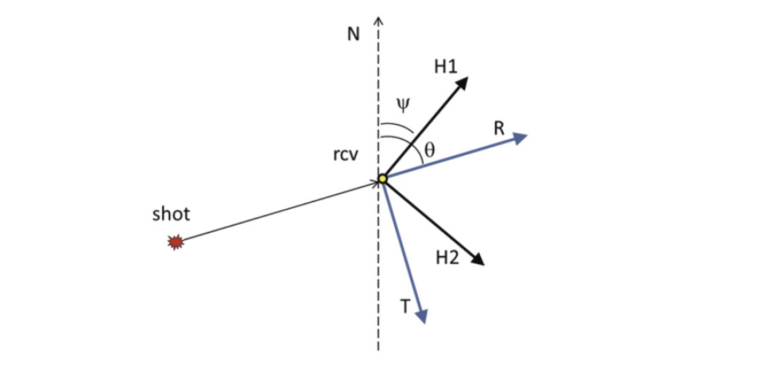
The geometry for orientation analysis is illustrated in Figure 1. Suppose we assume that the orientation of H1 is known to be Ψ, and that H2 is 90° clockwise from H1. Then for shots j=1, …, N with shot-receiver azimuth of θ_j , we can calculate the corresponding radial and transverse data as

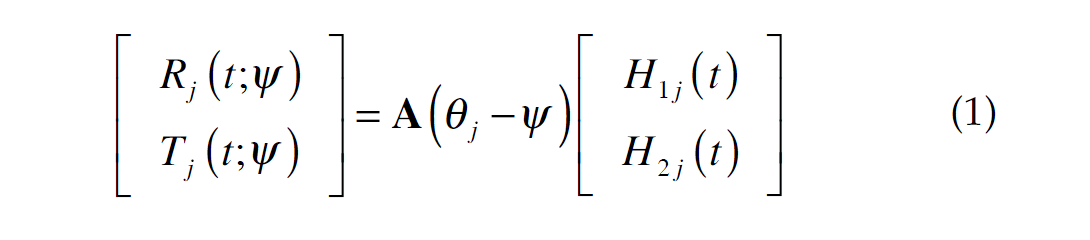
where H_1j(t), H_2j(t) are the H1 and H2 component records from shot j, and A is a rotation matrix

First breaks on R are assumed to be P-wave arrivals which should correlate maximally with the vertical component, V. This should apply for all shots into the receiver and we can construct a correlation function:

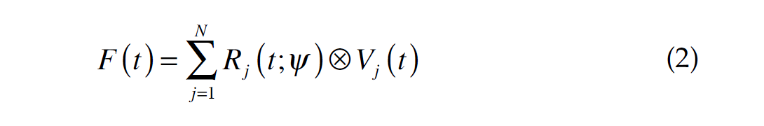
Where V_j is the vertical phone record for shot j. Ideally, the correlation is only performed over a window which contains first arrival data, to avoid contamination from reflections which may have been influenced by anisotropy. Now, regarding the receiver orientation Ψ as an unknown in equation (2) we search for a value of Ψ which maximizes F(t).

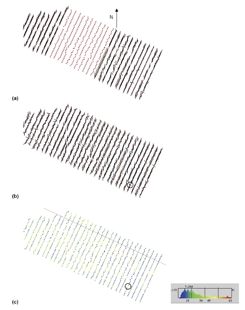
In the Kerrobert survey illustrated in figure 2, and later shown as our case study, the orientations of some of the receivers were measured after the survey was acquired (the receivers with no line segments in the figure had already been picked up). There was enough variance from the nominal orientation (magnetic North) that we decided to estimate orientations of all the receivers from the data, providing an opportunity to compare measured and estimated values where available.

The method described above for orientation analysis is based on the assumption that first breaks measured on both vertical and horizontal components are radially oriented P-wave arrivals. This assumption warrants some scrutiny, as it neglects near surface effects such as anisotropy and scattering. However, we found the analysis to be fairly robust when applied over many shots for each receiver.

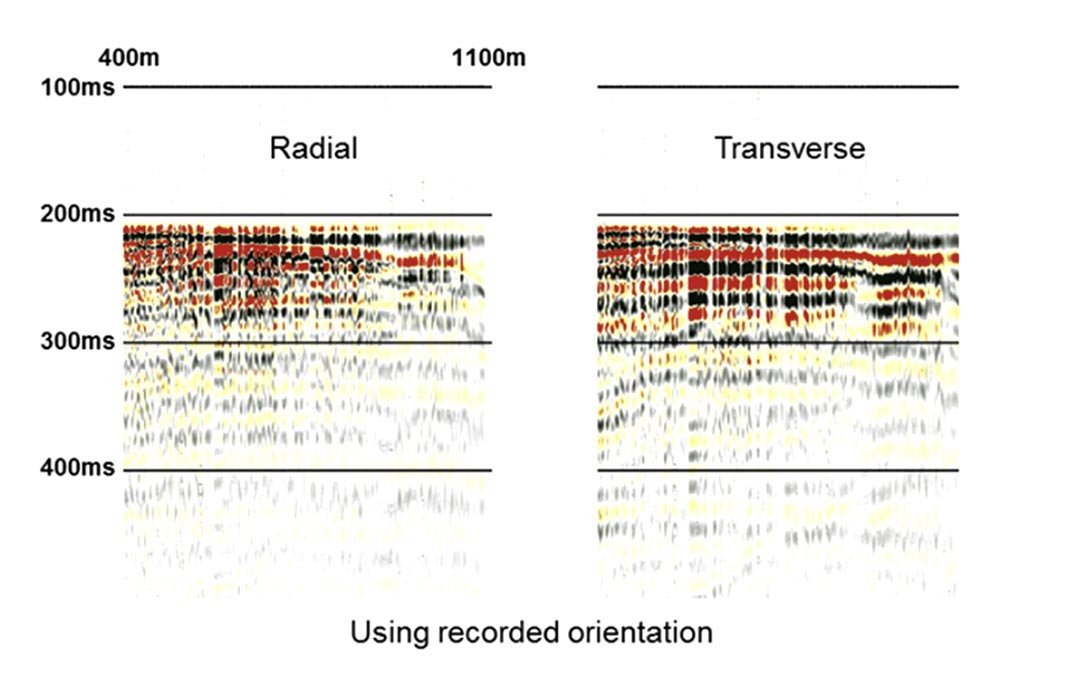
We can also perform the maximization of F(t) in equation (2) for each shot separately. The resulting estimates of Ψ have some scatter and the standard deviation of these is used to obtain an error estimate. Because these single shot measurements are quite noisy, the resulting standard deviation is generally larger than our actual errors, but is nevertheless useful to identify suspect locations. Figure 2(c) shows the error measurements for the orientations estimate in figure 2(b). We then visually compared the radial and transverse rotated data using the orientations which were recorded with those estimated by our method, at a number of locations including both high and low error spots. An example is indicated by the circles in figure 2(b) and (c), where the error QC was about 43°. Figure 3 shows the shallow data for this location, for offsets from 400m to 1100m, after flattening on first breaks and bulk shifting by 200ms. The analysis was performed on first arrival energy above 250ms on the shifted data, and over offsets up to 1100m. At this location, the estimated orientation deviates from the recorded orientation by 47°, giving rise to significant differences between the resulting rotations. The rotation to radial and transverse indicates a more plausible distribution of first break energy (higher on radial, lower on transverse) when the estimated orientation is used. We found that in general the orientations estimated from first breaks were at least as plausible as the recorded ones. Ultimately, we processed the entire dataset with the estimated values.

Shear-wave Splitting Analysis

Shear-wave splitting analysis can be viewed as a two-step process: first, estimate the azimuth of the S1 direction, and; second, estimate the time-delay between S1 and S2. Typically the transverse component is used to estimate the S1 azimuth, based on the azimuthal position of polarity flips or using an amplitude fitting approach (see for example Li, 1998). We refer to this as the T-only method.

However, amplitude information from the radial can also be incorporated in the process. We describe an algorithm to do this, based upon the theoretical form of the radial and transverse amplitude variations for an S1 direction ϕ, and N traces with radial directions θ_i . Assuming there are two time functions A₁(t) and A₂(t) which correspond to the S1 and S2 reflected amplitudes, then the radial and transverse amplitudes R(t, θ_i ) and T(t, θ_i ) can be written as

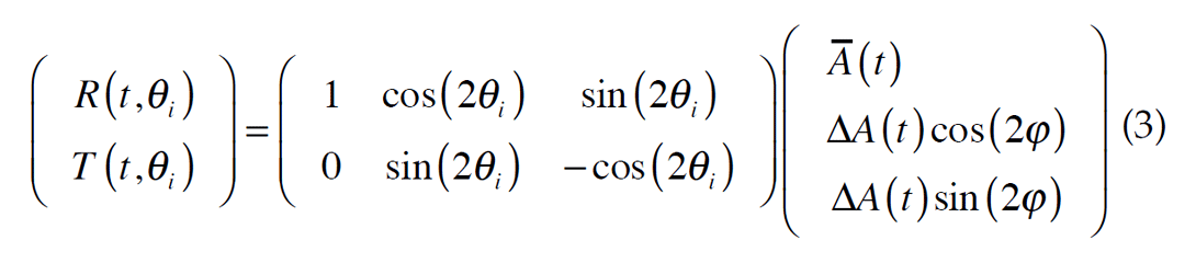
for i = 1, ..., N, where A(t) = ½ [A₁(t) + A₂(t)]

and ΔA(t) = ½ [A₁(t) – A₂(t)] .

Equation (3) can be written in matrix form as

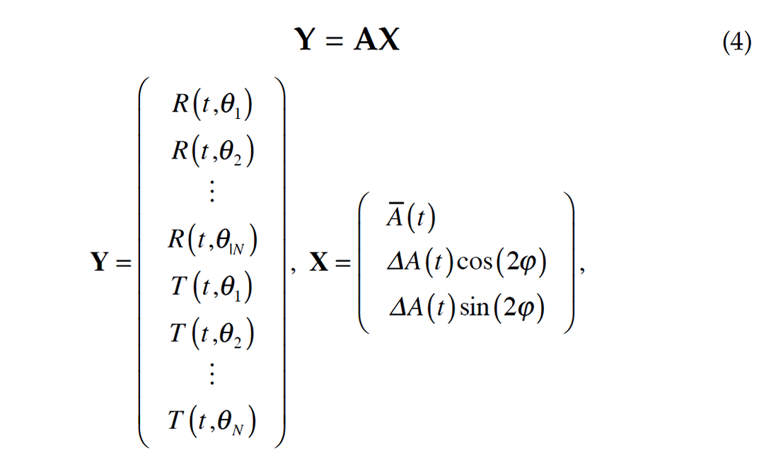
and

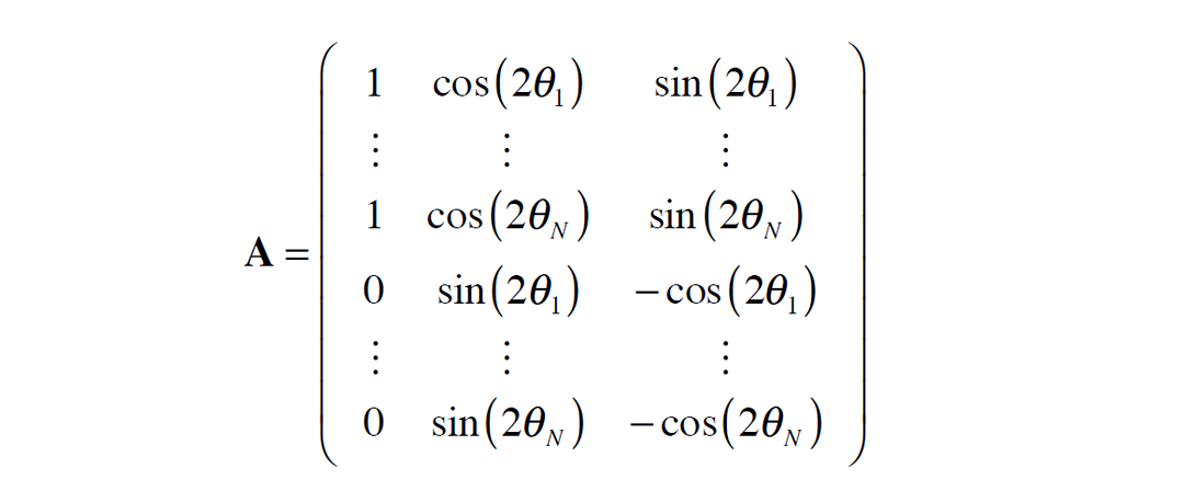
which can be inverted, provided N ≥ 2, to give the usual leastsquares estimate

The second and third terms of the solution vector X can then be combined to determine ϕ. We refer to this as the R+T method.

What is the advantage in using both radial and transverse as opposed to transverse alone? A common assumption is that, since the signal-to-noise ratio on the radial is higher than on the transverse, then an estimate using radial data in addition to transverse will be more robust. However, equation (3) makes it clear that the signal of interest is the deviation ΔA(t) from the background amplitude A(t). This deviation signal is no stronger (on average) on radial than it is on transverse. However, it does have a different sensitivity to the azimuth distribution, and so may help in areas where the azimuth distribution is poor.

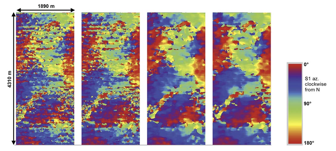
Figure 4 shows a comparison of S1 azimuth estimates measured on a heavy oil dataset at the Devonian level (about 1 second PS time) using 5x5 and 11x11 superbin sizes between T-only and R+T based methods. The receiver line spacing for this survey is 150m, which causes a noticeable acquisition footprint that contaminates the analysis results for shallow targets. As is seen in figure 4, for 5x5 superbin sizes, the footprint is somewhat reduced using the R+T method compared to the T-only method. However, if the superbin size is increased to 11x11, which is necessary to remove the footprint satisfactorily, then both methods perform equally well.

For the Kerrobert data, which had tighter acquisition parameters so that footprint was not a significant problem, we utilized analysis based on transverse component only.

P-S1 and P-S2 versus R’

There are two alternative ways to image the PS data after shearwave splitting analysis.

Perhaps the most obvious is to rotate data to S1 and S2 directions and image these two datasets (P-S1 and P-S2) separately. This is not as straightforward as it first sounds, as both P-S1 and P-S2 have azimuthal amplitude variations related to the sourcereceiver azimuth, including polarity changes. These must be dealt with appropriately, for example by the weighted stacking method of Bale et al. (2000). In this approach the P-S2 can be left in delayed time, or shifted to match P-S1.

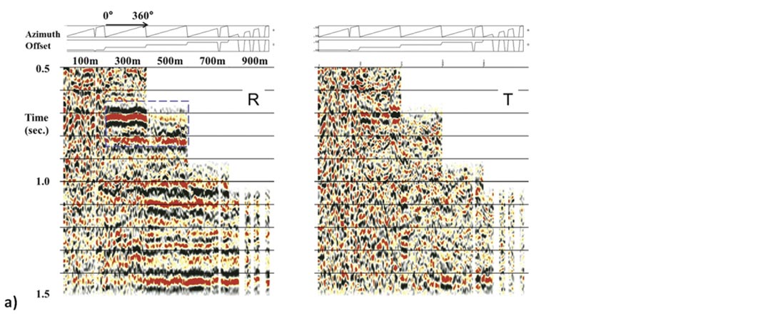
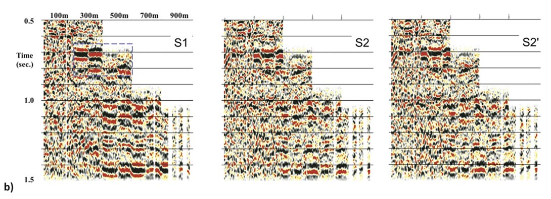
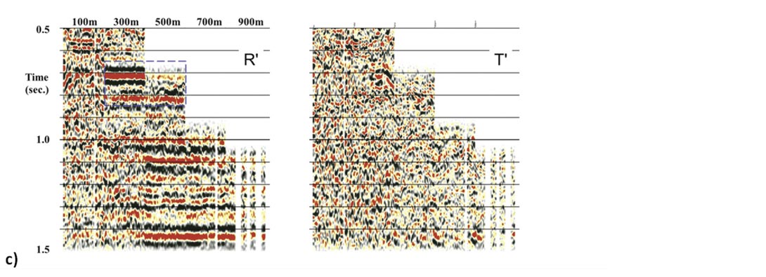
The alternative approach is to shift the P-S2 data to match P-S1 first and rotate back to the radial-transverse coordinate system. The resulting data may be referred to as radial-prime and transverse- prime (R’ and T’). This procedure is illustrated in figure 5, using the Kerrobert dataset shown later as our case study.

In order to layer strip through multiple layers, it is necessary to compute R’ and T’ for each layer in succession, in order to perform analysis for the subsequent layer. Often the R’ dataset is the most suitable for the final goal of imaging the reservoir.

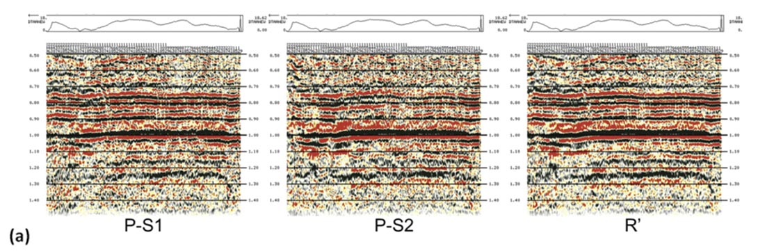
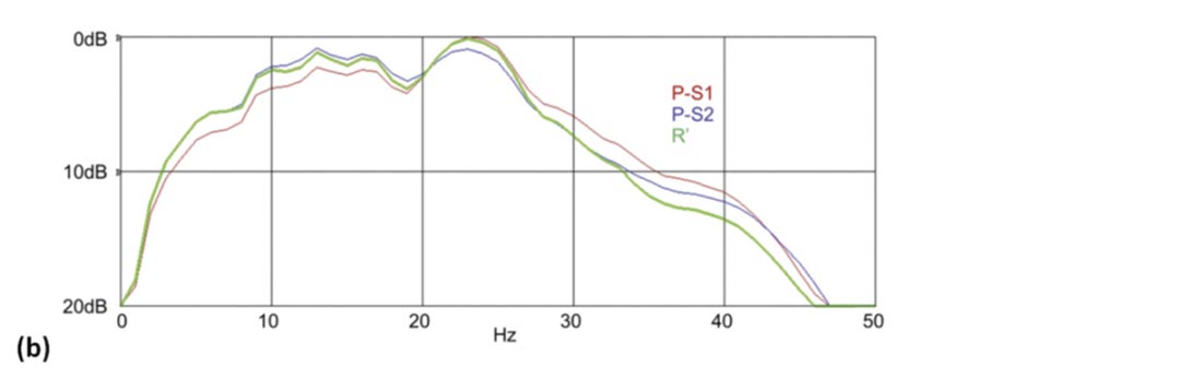
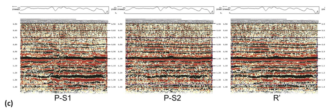
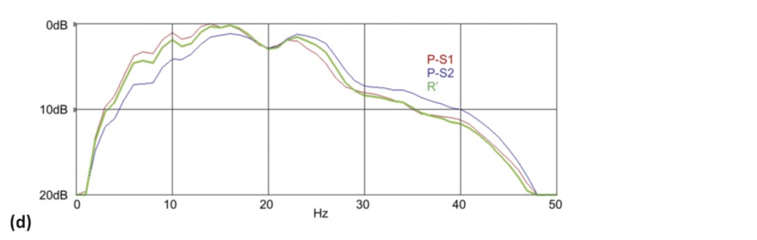
Nevertheless, there can be advantages in analysis of P-S1 and PS2 images separately, in particular for amplitude subtleties or spectral response. Figure 6 shows a comparison of data from the same heavy oil survey used in figure 4, processed for P-S1 and P-S2 images, and compared with a R’ image. Figure 6(a) shows a portion of the image from one line, while figure 6(b) compares the amplitude spectra for the three images. What is notable is that the P-S1 image is richer in the higher frequencies while the P-S2 is biased towards lower frequencies. This suggests (assuming equivalent reflectivity responses) that there is some degree of differential attenuation being observed between the two modes, with the P-S2 mode having greater frequency dependent losses than the PS1 mode. We have observed this to be fairly prevalent within this dataset. However, there are examples elsewhere of the reverse behavior, as shown in figure 6(c). In both cases, the R’ spectrum benefits from the combined contributions of P-S1 and P-S2.

Case Study: Splitting Analysis for Recovery Monitoring over a THAI Reservoir

The Kerrobert field, near the town of the same name in Saskatchewan, is the location of the first commercial THAI operation in Canada (two THAI pilots have been operated in Canada since 2005). The reservoir of interest is ~750m deep and consists of well consolidated sands that range in thickness from 15-30m. The caprock in this area consists of over 50m of marine shales in the Mannville group, providing thick continuous containment of the process. The reservoir has been developed using cold production methods, however, as in most heavy oil reservoirs, primary recovery is quite low at 1.5% of original oil in place. The pilot phase for THAI utilized two wells (KP/KA 1-2) from 2009-2011 with another 10 wells drilled for commercial development in early 2011 (KP/KA 3-12). The Kerrobert expansion wells were brought online in July-August 2011, while the first 3C seismic shoot occurred in October 2011.

The THAI process utilizes one air injector/horizontal producer pair for insitu combustion. A detailed overview of the THAI process can be found in Kendall (2009) and Wikel et al. (2012). We know from reservoir modeling and previous piloting experience that the THAI front and its advancement change the pore pressure and fluid content within the reservoir as combustion progresses. It follows that a change in fluid state, gas content, and an increase in pore pressure with increased air injection should result in a change in seismic response over time and should produce 3C anomalies at the time of the shoot. It is believed that stress is the dominant factor in shear wave splitting anomalies within the reservoir, however, small contributions in splitting from fluid phase changes cannot be ruled out.

4D-3C seismic was chosen as the primary method for monitoring these variations through time, as the changes throughout the reservoir and caprock will be heterogeneous, meaning that simple wellbore monitoring alone is insufficient. The examples below are the baseline for future 3C shoots.

Shear-wave splitting analysis at Kerrobert was performed using four layers, selected using a combination of stress analysis objectives and signal quality considerations. These layers correspond to overburden, two layers above the caprock (the second layer bounded at the bottom by the caprock) and a final layer over the reservoir. Figure 7 shows splitting analysis results from the overburden and the layer bounded by the caprock. Figures 8 and 9 are focused on the reservoir analysis.

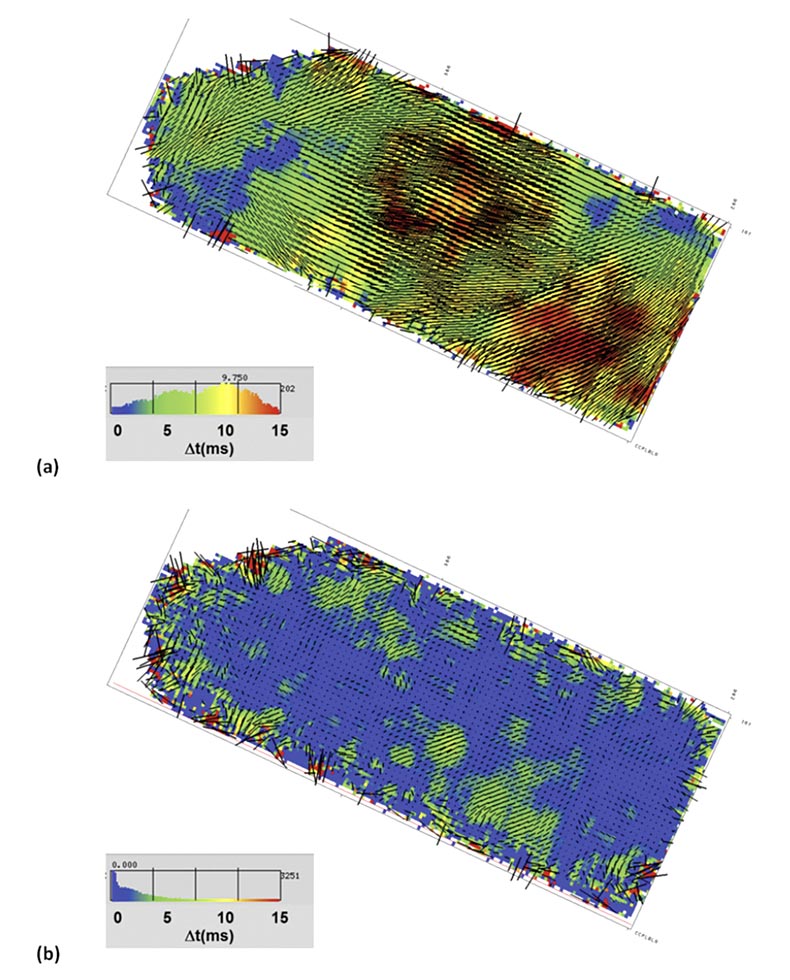
As has been observed numerous times in heavy-oil PS data (Whale et al., 2009; and Cary et al., 2010) the most significant Swave anisotropy effect, at least in a raw time-delay sense, comes from the near surface, as seen in figure 7a. The measured overburden anisotropy has a mode around 10ms which, for analysis over 750ms from surface, corresponds to an average S-wave anisotropy of about 1.3%. Though this is not high in percentage terms, it can have a noticeable impact on imaging if not corrected for. Of course, layer stripping of this layer is also critical for obtaining meaningful analysis results for subsequent layers. The area between overburden and caprock was divided into two layers. Results from the second of these, after correction for the first, are shown in figure 7b. This might be characterized as largely isotropic with isolated pockets of measureable splitting.

We now turn our attention to the final layer, which was analyzed after layer stripping overburden and caprock layers.

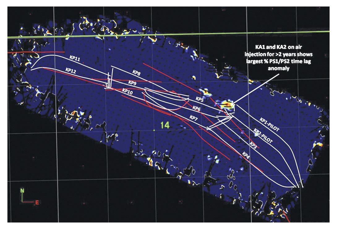
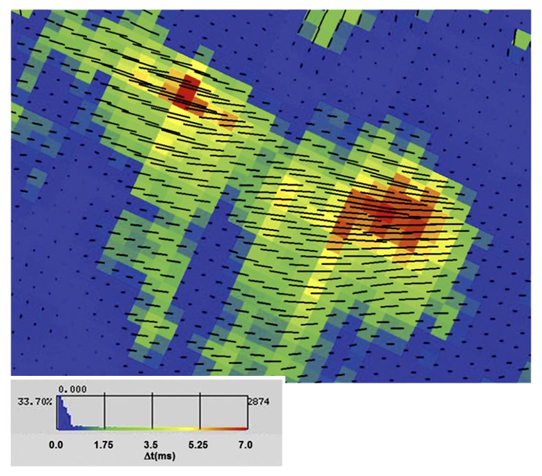
Figure 8 shows the PS1/PS2 time lag with the PS1 direction referenced to true north overlaying the horizon as a vector (vector size scaled by time lag). In this display we normalize the time lag (~7ms) by the time interval from the previous layer to this one (75ms), to get the percent anisotropy over the reservoir. Figure 9 shows a zoom of anomaly in figure 8, as raw time lags (not normalized), with a different colour scale to highlight the PS1 vectors. As shown in figure 8 and 9 there is a large anomaly which shows 10% anisotropy over the window. This is a large anomaly, given that layer stripping was performed on three layers overlying this reservoir. In addition, this large PS time lag anomaly is located at the bottomhole location of the two air injectors in the field that have injected the largest volumes of air and have been implementing THAI for the longest period in the field (KA/KP 1-2). These two air injectors and horizontal producers were the location of the THAI pilot in this field, as noted.

Conclusions

PS data is proving useful for identification of stress variation in the near surface over heavy oil reservoirs, in the absence of natural fracturing. To enable this analysis, it is important to accurately measure receiver orientation, or, if necessary, to estimate it as well as possible from the data.

The first step in splitting analysis is to estimate S1 azimuth, which is typically done using the transverse component alone (T-only). We found some marginal benefit to a method using both radial and transverse (R+T), which reduced the footprint on azimuth estimates with large receiver line intervals, but not enough to obviate the need for substantial superbinning.

A comparison of P-S1 and P-S2 data after weighted stacking indicates possible differential attenuation between these modes and that the R’ spectrum benefits from the combination of the two modes.

The results of this type of analysis, when processed correctly, are crucial for monitoring reservoir changes that may not be apparent on PP data only. This includes monitoring overburden and reservoir changes via converted wave splitting. Monitoring in this fashion provides areal coverage that cannot be achieved with wellbore monitoring alone. 3C methods are well suited for most thermal and EOR processes where appreciable reservoir changes occur, such as CO2 floods, cyclic steam stimulation (CSS), and steam assisted gravity drainage (SAGD).

Acknowledgements

We thank Key Seismic Solutions and Petrobank Energy and Resources for permission to publish this work. We also would like to thank Jeff Deere for his careful review.