Preserving sensor vector fidelity using automated multicomponent receiver-azimuth detection

Abstract

P-S converted-wave energy is recorded mainly on the two lateral components of the receiver. Conventional processing of converted-wave energy includes rotation of these laterally polarized data measurements into radial and transverse coordinates. To do this properly, knowledge of the in-situ receiver orientation is essential. However, substantial errors in the recorded receiver azimuth can arise in practice, causing undesirable ‘leakage’ of radial energy onto the transverse component. This in turn could be misinterpreted, for example, either as evidence of shear-wave splitting or out-ofplane reflection energy.

To address this problem, we developed a high-fidelity method for automatically detecting the receiver azimuths. This new method is based on multicomponent, azimuthal information extracted from the P-wave first-break energy, which is present on all three components. For each receiver ensemble, and for each shot-receiver azimuth, a measure of the amplitude over the samples following the first-break pick up to the first detected zero-crossing is determined. For a given receiver, and for each lateral component, these values are subsequently used in conjunction with an orthogonality constraint as weights to determine the best-fit orientation for that receiver; a subsequent global analysis of the results yields a robust probability measure indicating the confidence level associated with the resulting receiver-azimuth estimate.

Introduction

Motivation

Typically, P-S converted-wave energy is primarily recorded on the two lateral (H1 and H2) components of the receiver. This occurs for two reasons. Firstly, velocity tends to increase with depth, which, according to Snell’s law, causes rays to bend progressively toward the vertical as depth decreases. Secondly, shear waves typically propagate much more slowly than the compressional waves which generate them upon reflection from an interface. It follows again from Snell’s law that the conversion point is laterally closer to the receiver than the midpoint between source and receiver. Thus, converted waves tend to arrive at the receiver along a more vertical trajectory than pure P-wave reflections; hence the converted shear-wave particle motion, which oscillates in a direction perpendicular to the trajectory, is mainly recorded on the lateral components.

Conventional processing of converted-wave energy includes rotation of these laterally polarized data into radial and transverse coordinates. To properly accomplish this change of coordinates, knowledge of the in-situ receiver orientation is essential. However, substantial errors in the recorded receiver azimuth frequently arise in practice, and these errors spuriously manifest themselves as radially polarized energy on the transverse component, thereby degrading the fidelity of the signal recording. Further complications include potential misinterpretation of this energy seepage on the transverse component, for example, either as evidence of out-of-plane reflection energy, or, perhaps worse, shear-wave splitting. Indeed, Cary (2002) used forward-modelling of convertedwave data with and without minimal geometry errors (on the order of 5%) to show that such errors can generate the same effects as shear-wave splitting on limited azimuth stacks.

Solution

To address this so-called ‘leakage’ problem, we have developed a robust, high-fidelity algorithm for automatically detecting the receiver azimuths from 3C-3D experiments.

We begin by discussing the theory behind the basic assumption of our method; namely, that first-break energy is measurable on the two lateral receiver components in the form of compressional head waves. We then discuss our method, providing details on how source-receiver azimuthal information can be extracted from this P-wave first-break energy to detect receiver orientation. Finally, as part of our method, we describe how to construct a probability measure which indicates the confidence level associated with the resulting receiver azimuth estimate. We follow up with some results on real data which clearly demonstrate both the validity and value of our method.

Theory

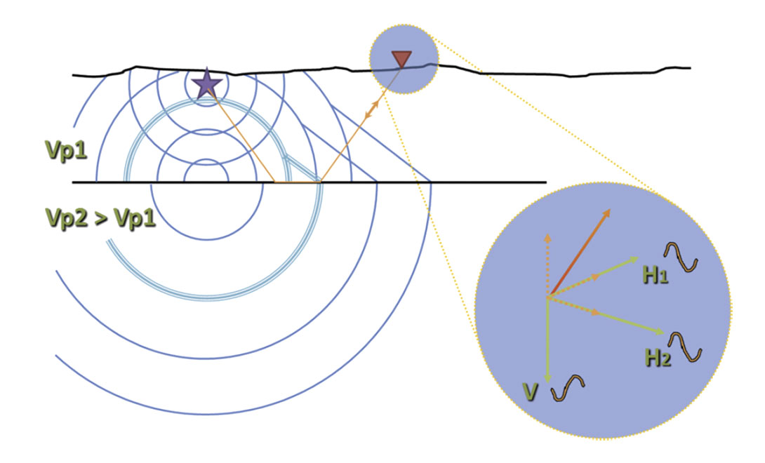
The head waves which typically appear as first breaks in land seismic data are commonly referred to as ‘refractions’. This can be misleading, since a refraction is really any change in direction of a wave due to a change in its propagation medium. Perhaps the term is a shortening of the concept of ‘post-critical refractions’ (see Lines and Newrick, 2009, Chapter 4). Figure 1 illustrates this phenomenon of post-critical-angle head-wave generation. A snapshot of the head wave is depicted as the linear wavefront connecting the reflected and transmitted wavefronts (all in turquoise triplicates), together with the ray-path (orange) associated with these particular source and receiver locations. Essentially, the up-going head wave arises as a consequence of the transmitted wavefield propagating faster than the incident wavefield, and because continuity of the wavefronts must be maintained for physical reasons (see Grant and West, 1965 for a more detailed explanation). We can think of the head wave as being generated by a point source propagating along the interface at the speed of the lower medium.

The expanded view of the receiver in Figure 1 illustrates the projections (dashed orange) of the incident P-wave particle motion (red) onto all three measurement components (lime). This happens simply because the compressional head-wave is polarized in the direction of propagation, which evidently is not vertical. In this example, a peak in the wavefront is recorded as a trough on the vertical component, while peaks are measured as peaks on the lateral components. The projection onto a lateral component vanishes only when the component is perpendicular to the plane of propagation.

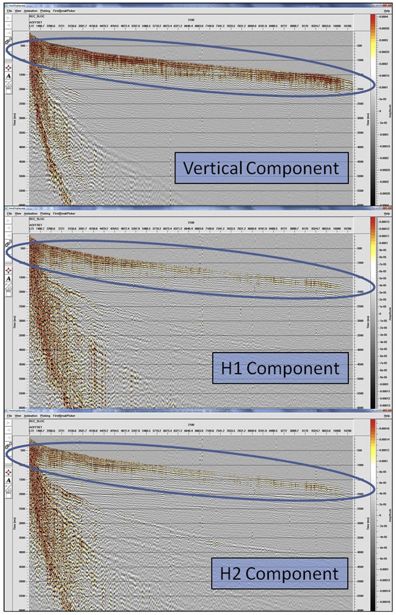
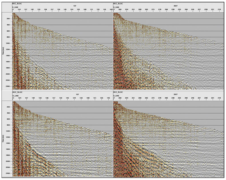
The existence of P-wave refraction energy on all components is clearly evidenced by the real data example shown in Figure 2. Each of the three components is displayed for a fixed receiver ensemble. The data has been tilt-corrected but no rotation has been applied.

Method

Our method relies on the ability to pick the first-break head waves on the vertical component of the data, and makes use of the fact that these first breaks – as we have shown above – are also measured on the two lateral components of the receiver.

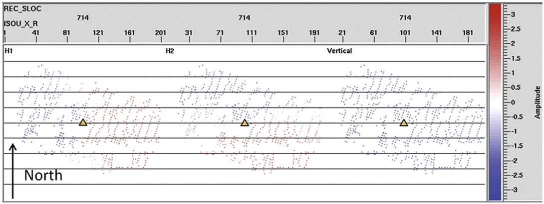
First, analysis is performed on each of the lateral components of the data. For this step, we developed robust code for detecting the first zero-crossing following each first-break pick, and storing an amplitude measure (mean, max, or signed count) associated with the samples between the first break pick and the detected zero-crossing. This process is repeated on each component for all traces. These first-break amplitude measures are displayed in map view for each of the three receiver components in Figure 3.

For the next step, we further developed the code to estimate the orientation of each receiver, with input based on receiver ensembles. For each receiver ensemble, and for each shot location within the current ensemble, the code constructs an objective function as it scans over all trial azimuths from 0° to 360°. The first-break amplitude measure obtained in the previous step is used to weight the contribution of each trace, based on its sourcereceiver azimuth and the current test azimuth for the receiver. Put another way, the best-fit azimuth for each component is determined by considering, for each trial azimuth, the inner product of a 2D step function, rotated by the trial azimuth, with the data points in the corresponding map as depicted in Figure 3. The best-fit step function will be 90° out of phase with the actual receiver-component orientation. Thus the problem is reduced to that of simple edge-detection – one of the basic tools of computer vision (see e.g., Shapiro and Stockman, 2001).

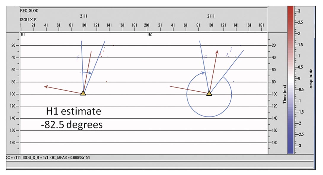
The final stage of the method involves global analysis of the objective function in order to construct a probability measure, which is ultimately used to decide whether to assign an azimuth correction to each receiver. In the ideal case where we have a receiver with a well-populated, uniform distribution of shotreceiver azimuths, we expect the objective function for that receiver to have an obvious global maximum. This is not typical however, so we need to consider the case where the global maximum occurs over a nontrivial range of azimuths, such as that depicted in Figure 7 below. Another factor to consider is the number of data points involved in the analysis. In both cases, we opted to penalize the objective function by normalizing it by a power of the quantity involved: the number of contiguous maxima and the number of data points. We further penalized the function by the number of connected components in the set of maxima (typically this is redundant). A final normalization by the global maximum over all receivers yields the probability measure we were seeking.

Results

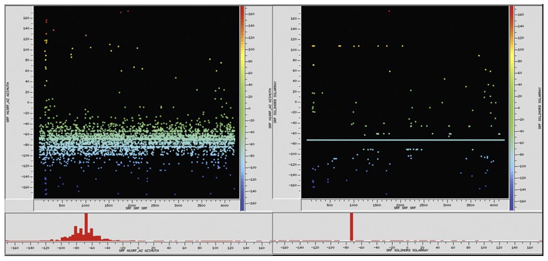
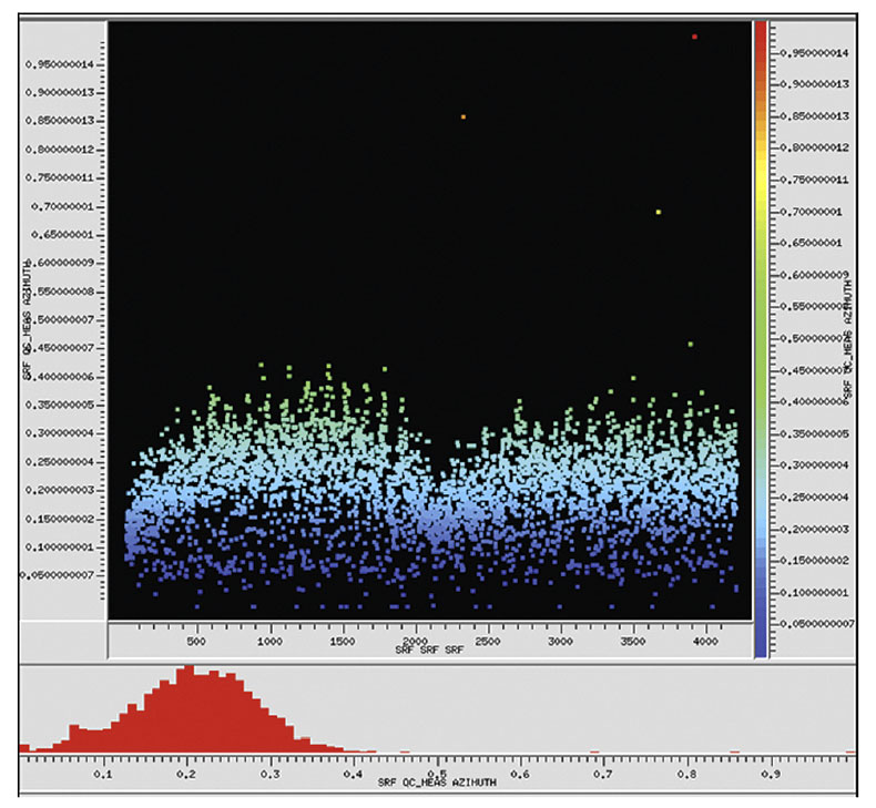
Figure 4 illustrates the results of running the automated azimuth detector on all receivers in the survey (left) vs. the nominal azimuths (right). The H1-component azimuths are displayed in both plots as a function of receiver number. As expected, the detected azimuths are nearly normally distributed. The results also suggest the algorithm is unbiased, since the mean detected azimuth (-72°) agrees precisely with the mean nominal direction, which also happens to be the dominant receiver-line azimuth for the survey.

Transverse-component, moveout-corrected, and muted receiver gathers are displayed in Figure 5. The columns correspond to two distinct receivers, and the rows correspond to rotating the data to radial and transverse coordinates by: 1) the automatically detected azimuth (top row); and 2) the nominal azimuth (bottom row). The estimated azimuth errors are -90° (left column) and 57° (right column) respectively. As desired, reflection events are virtually absent in the azimuthdetected results, while considerable coherent energy remains on the corresponding nominal result. Energy from the shear-mode head waves is evident in the lower left-hand corner of both results; as expected, this energy is also stronger and much more coherent in the nominal results.

Conclusions

Conventional processing of converted-wave energy includes rotation of primarily laterally polarized data measurements into radial and transverse coordinates, which requires knowledge of the in-situ receiver orientation; however, errors in the recorded receiver azimuth are commonplace, which ultimately leads to undesirable leakage of radial energy onto the transverse component. This contamination can be misinterpreted, for example, either as evidence of shear-wave splitting or out-of-plane reflection energy.

To address this problem, we developed a high-fidelity method for automatically detecting the receiver azimuths. We based this new method on multicomponent, azimuthal information extracted from the P-wave first-break energy, which we showed is present on all three components. For each receiver ensemble, and for each shot-receiver azimuth, we determined a measure of the amplitude over the samples following the first-break pick up to the first detected zero-crossing. For a given receiver, and for each lateral component, these values were subsequently used in conjunction with an orthogonality constraint as weights to determine the best-fit orientation for that receiver; a subsequent global analysis of the results yielded a conservative probability measure indicating the confidence level associated with the resulting receiver-azimuth estimate.

Acknowledgements

We thank Sensor Geophysical Ltd. (a Global Geophysical Services Company) for permission to publish these results.