Mapping the Distribution of Permafrost using the Resolve Airborne EM System: Klondike Highway, Yukon, Canada

Introduction

Changes in permafrost distribution in northern regions of North America are related to hydrogeological processes, climate, and ecosystems (Minsley et al., 2012). In particular, increased thawing due to warmer temperatures alters the permafrost distribution (Minsley et al., 2012, Oldeberger et al., 2015). This can lead to enhancement of surface-groundwater interactions that contribute to surface flow (Bense et al., 2009; Walvoord and Striegl, 2007) which leads to differential melting of the permafrost. Differential melting generates safety problems for Yukon highways, for example potholes and linear fractures. Costs for repairing features such as these can be significant. This paper presents the results of using an airborne EM survey to map the permafrost distribution along a section of the Klondike Highway.

Earlier investigations carried out to understand the distribution of permafrost along Yukon highways have focussed on traditional methods, for example: geological boreholes and ground geophysical surveys (Oldenberger et al., 2015; Golder Associates, 2013). These studies, along with the recent paper by Minsley et al. (2012) on the RESOLVE airborne electromagnetic method (AEM), show that geophysics methods that map subsurface resistivity can be used to determine permafrost distribution.

A RESOLVE airborne electromagnetic system was flown along the Flat Creek section of the Klondike highway a few kilometres south of the Dempster highway intersection. The locations of the areas flown are provided, along with a description of the airborne system. An interpretation of the permafrost thickness determined from the differential resistivity cross sections provided by CGG, the airborne contractor for the areas flown, is presented. Borehole information provided by the Yukon Highways and Public Works Department and photos of several slumping areas along the Klondike Highway are compared and analyzed with the airborne results. A conclusion section summarizes the main results of the study.

Location of survey

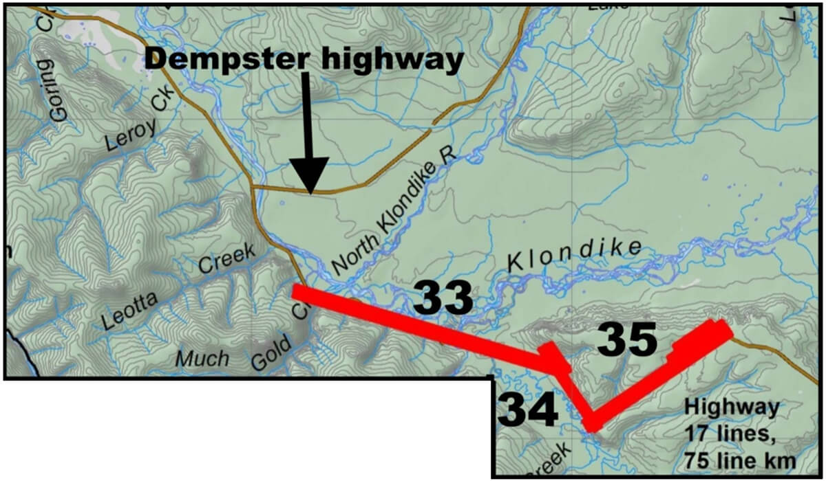
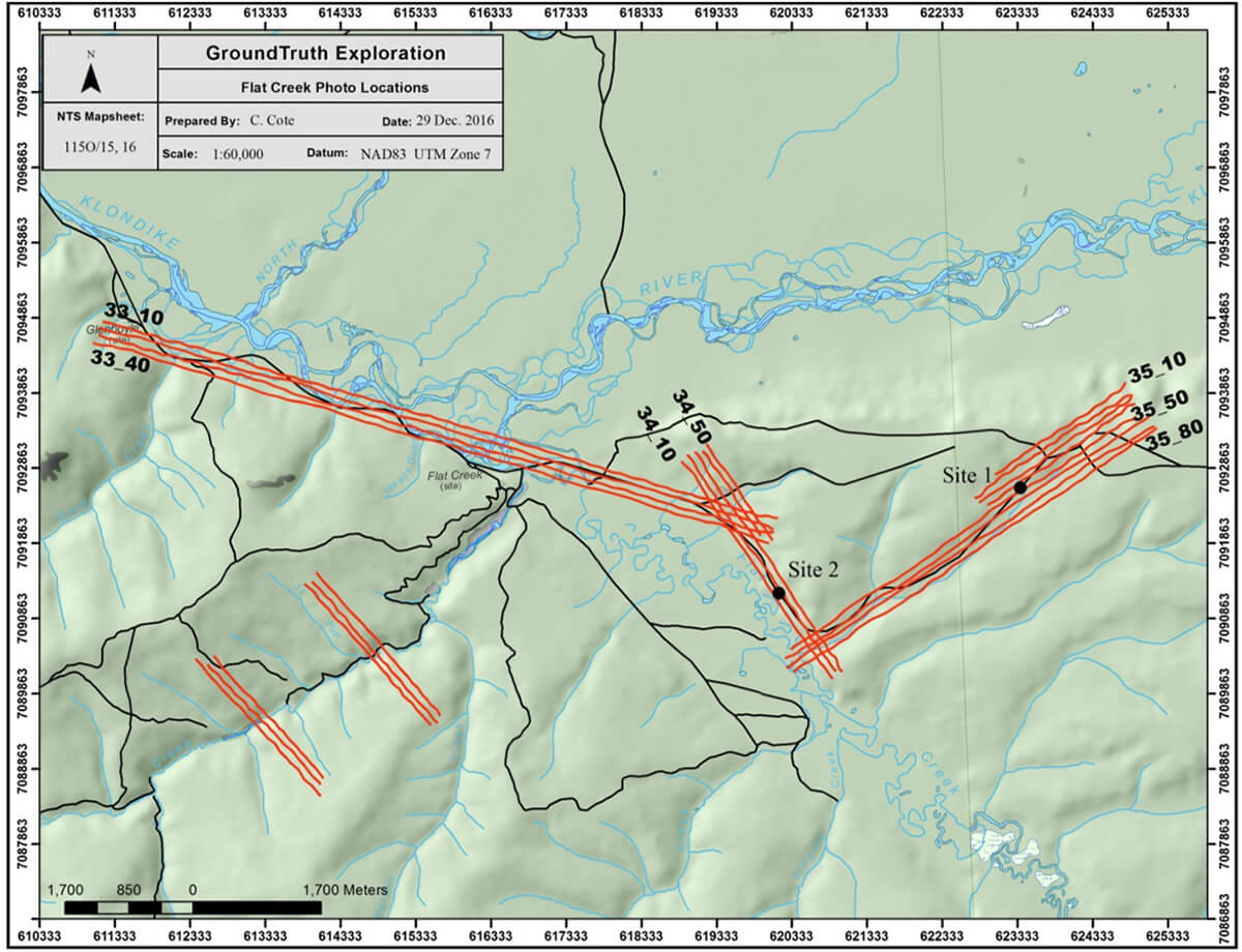
Figure 1 is a map showing the location of the 3 areas (33, 34 and 35) flown to map the permafrost distribution. The areas, which approximately follow the Klondike Highway, consist of 4 flight lines for area 33, 5 flight lines for area 34 and 8 flight lines for area 35 for a total of 17 flight lines or approximately 75 km of flying. Lines are flown parallel to each other approximately 50 to 100 m apart, depending on the location of power lines and other obstacles.

RESOLVE airborne EM system

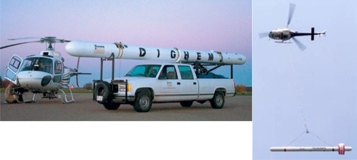
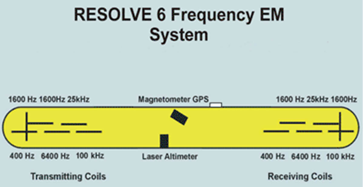
The RESOLVE airborne EM system is a frequency-domain helicopter EM system flown by CGG. It consists of a towed bird flown at a height of 30 m above the ground (Figure 2). The helicopter is flown approximately 30 m higher than the bird for safety. The bird contains 6 transmitter-receiver pairs, with 5 pairs oriented in the horizontal or coplanar configuration and one pair oriented in the vertical or coaxial configuration (Figure 3). The frequencies used for this survey were 400 Hz, 1800 Hz, 8200 Hz, 40 kHz and 140 kHz for the 5 coplanar configurations. The coaxial pair and the magnetic channels, although they were recorded, were not used for this investigation.

The electromagnetic receivers measure the voltage using Faraday's Law, i.e. the voltage is proportional to the time rate of change of the magnetic field. For each transmitter-receiver pair, the RESOLVE system measures the normalized voltage (VN) in parts per million (ppm). This is the ratio of the secondary voltage (VS) caused by conductors within the subsurface divided by the primary or free space voltage (VP) which is the voltage that comes directly from the transmitter (i.e. when there are no conductors present). Therefore, the normalized voltage is: VN = VS/VP. The secondary voltage measured in the receiver is produced through the process of electromagnetic induction (eddy currents in the subsurface) which produces a phase shift between the transmitter current and the measured receiver voltage. The part of the normalized voltage that is in-phase with the transmitted current is called the in-phase voltage and the part of the normalized voltage that is exactly 90 degrees out of phase with the transmitted voltage is called the quadrature voltage. These two voltages are measured in ppm because the primary voltage, which is the voltage coming directly from the transmitter to the receiver, is significantly larger than the secondary voltage that emanates from the subsurface.

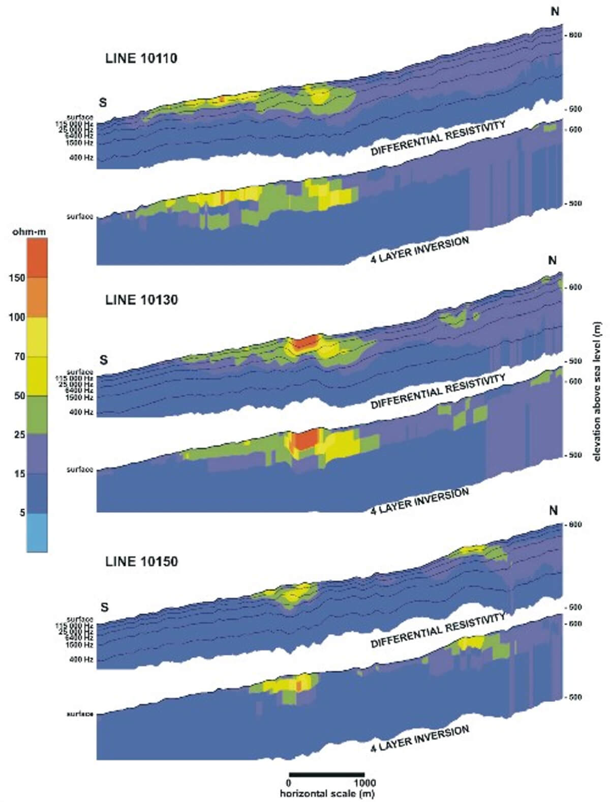
The normalized voltages are then converted to resistivity profiles and resistivity depth slices using the in-phase and quadrature values for all 5 frequencies. The simplest way is to generate differential resistivity sections (Sengpiel, 1983; Sengpiel and Sieman, 2000; Huang and Fraser,1996). Although not true inversions, they provide a fairly accurate representation of resistivity versus depth. One-dimensional multi-layer inversions are possible using the same set of data as well. Figure 4 is a comparison of a 4-layer 1D resistivity inversion and differential resistivity cross section for RESOLVE data from a gravel mapping study carried out in NE BC (Best et al., 2006). The two methods generate nearly identical results. The differential resistivity sections can be generated much faster and cheaper than layered earth inversions. Consequently, differential resistivity sections are used for this study.

AEM and ancillary data

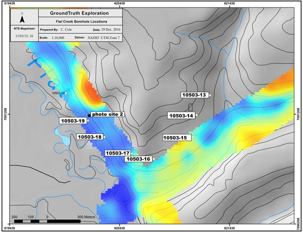
The products used to interpret the sub-surface resistivity distribution are resistivity cross sections and depth sections (5, 10, 20, 30, 40, 50, and 75 m) obtained from the differential resistivity computations. Note resistivity scale bars are not all identical. A reconnaissance visit to areas 34 and 35 provided photographic evidence of road slumping and potential failure at two sites; site 1 in area 35 and site 2 in area 34 (see Figure 5). In addition, Figure 6 shows the location of boreholes provided by the Yukon Department of Highways. Except for boreholes 10503-16 and 10503-19, the maximum depths of the boreholes are less than 7 m. Borehole 10503-15 reached a depth of 17.4 m and 10503-19 reached a depth of 24.7 m. Most boreholes had approximately 1.5 m of frozen ground at the beginning of the holes and shallower depths contained a mixture of sand, silt and gravel. Borehole 10503-19 had clayey material from approximately 15 m to the end of the hole at 24.7 m and borehole 10503-16 reached a very hard bedrock surface at approximately 17 m. No permafrost was encountered in borehole 10503-16.

Interpretation and integration of all the data

Figure 7 is a plot of different sediment types showing approximate ranges of resistivity values associated with frozen versus unfrozen material (Hoekstra et al, 1975, Palacky, 1987, Minsley et al., 2012). If the resistivity values of sand and gravel are above 500 ohm-m they are typically frozen within a permafrost area whereas for clay, the resistivity values above 200 ohm-m tend to be frozen. Partially and unfrozen sand and gravel have resistivity values that overlap those of frozen resistivity values, depending on water content of these sediments. Therefore, determining frozen versus unfrozen material can be difficult at times.

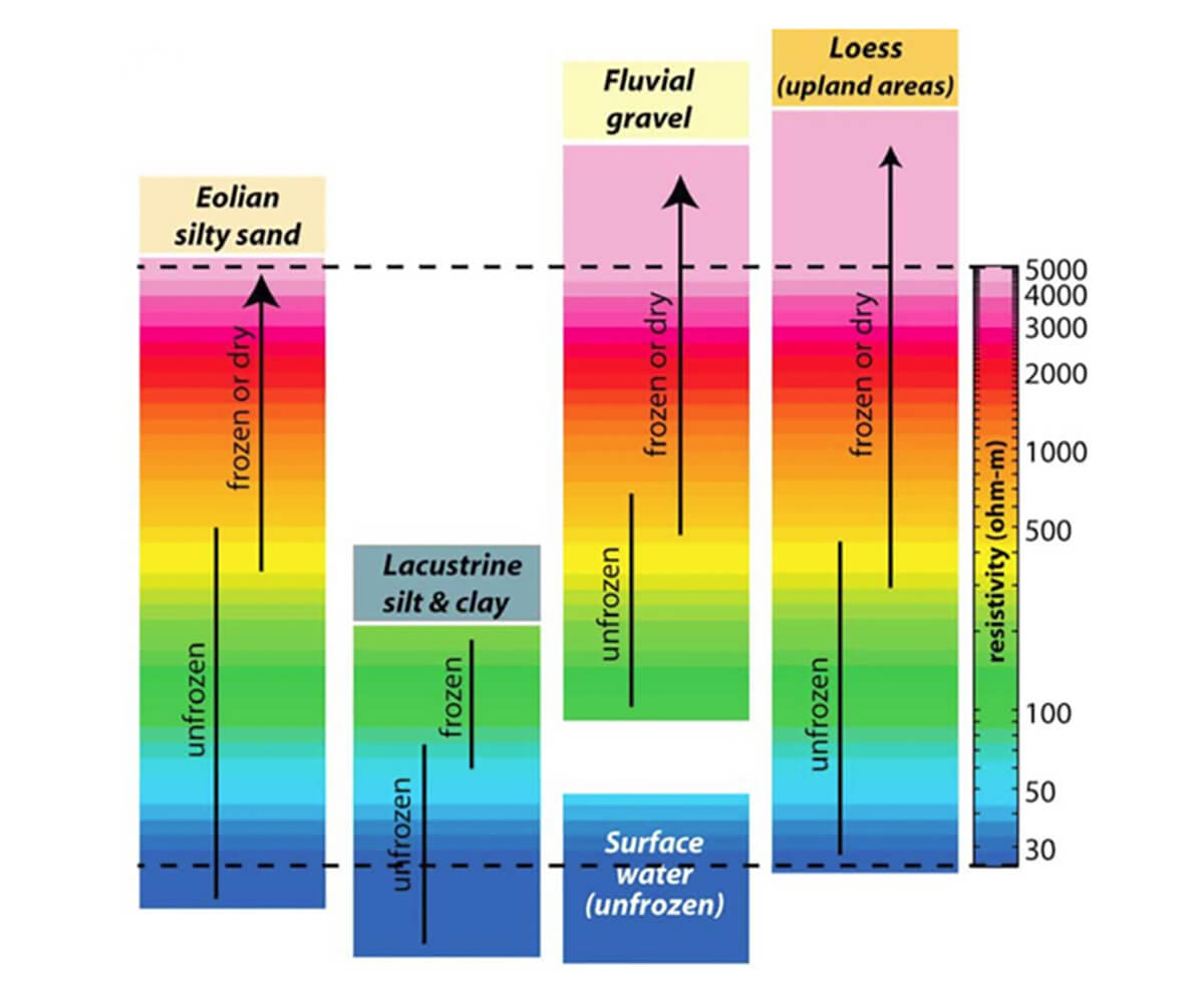
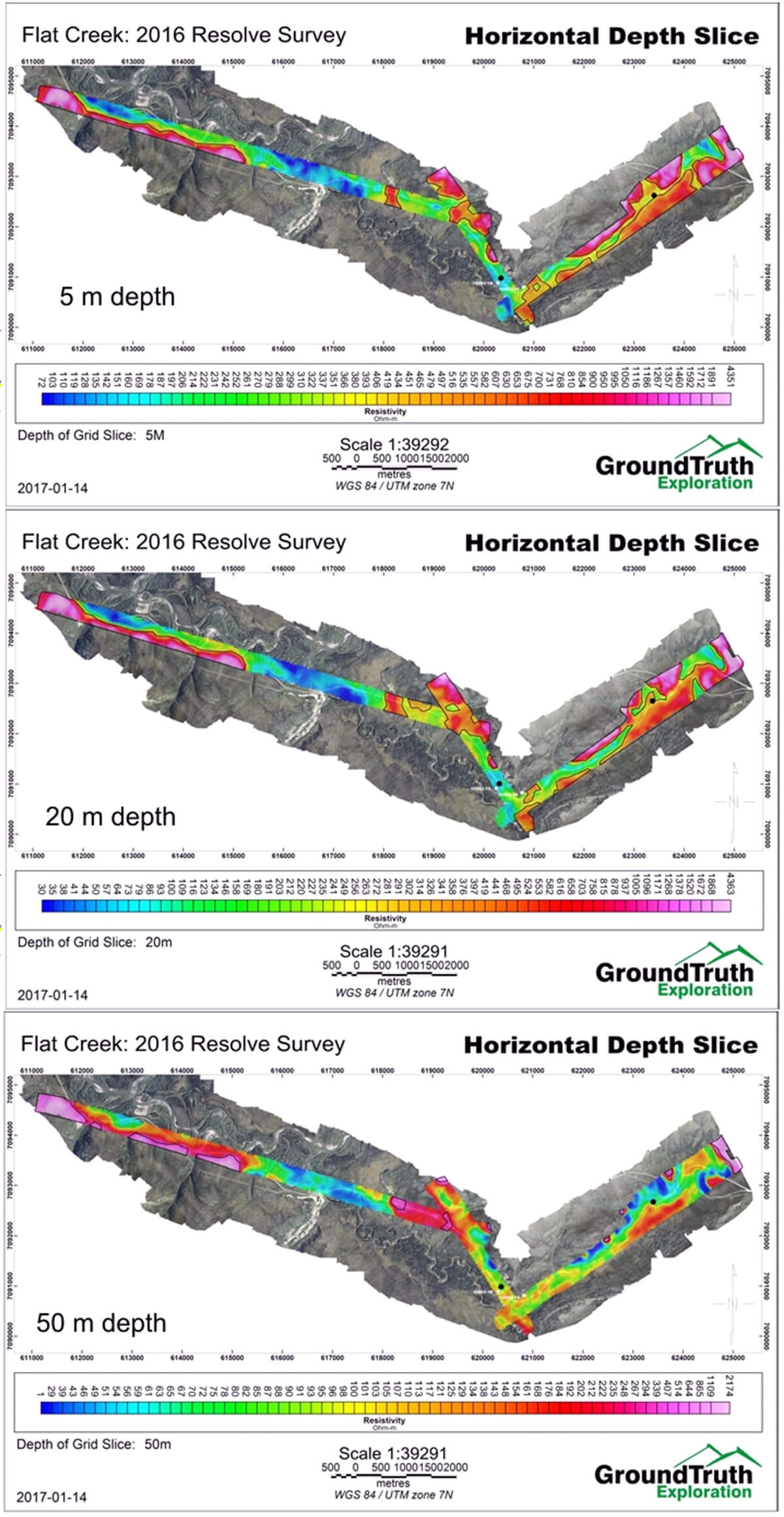
Figure 8 provides plots of 3 resistivity depth slices (5, 20 and 50 m depths) for areas 33, 34 and 35. These show that resistivity values change with depth. The black lines outlining higher resistivity regions are potential permafrost areas, except for the 50 m depth slice where the higher resistivity zones may indicate bedrock. Although there is no borehole calibration available for area 33, these higher resistivity zones indicate the south side of the NW region of area 33 consists of frozen ground to a depth of approximately 20 m. By 50 m depth, the higher resistivity zones are more likely associated with bedrock. The central section of area 33 is unfrozen ground and is directly associated with the creek seen near the middle of the zone. There is less permafrost in the SE section when compared with the NW section. However, these depth slices indicate there is some frozen ground in this region of area 33 as well. Areas 34 and 35 have borehole control. We shall only look at the flight lines closest to the two deeper boreholes (10503-16 and 10503-19) which are lines 35-50 and 34-10 respectively (Figure 9).

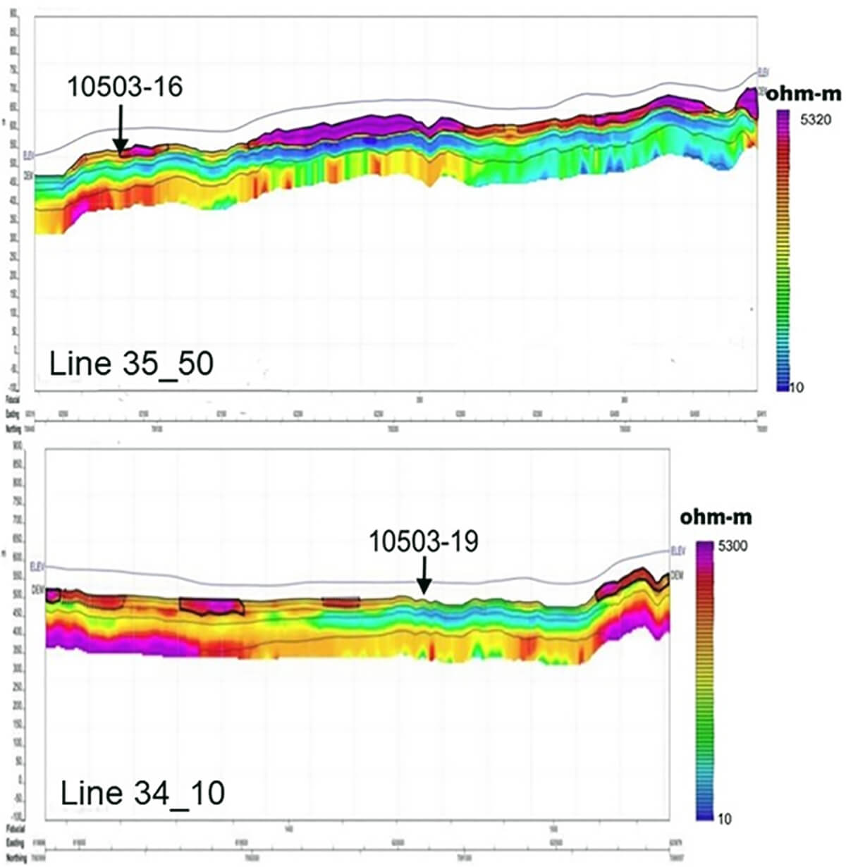
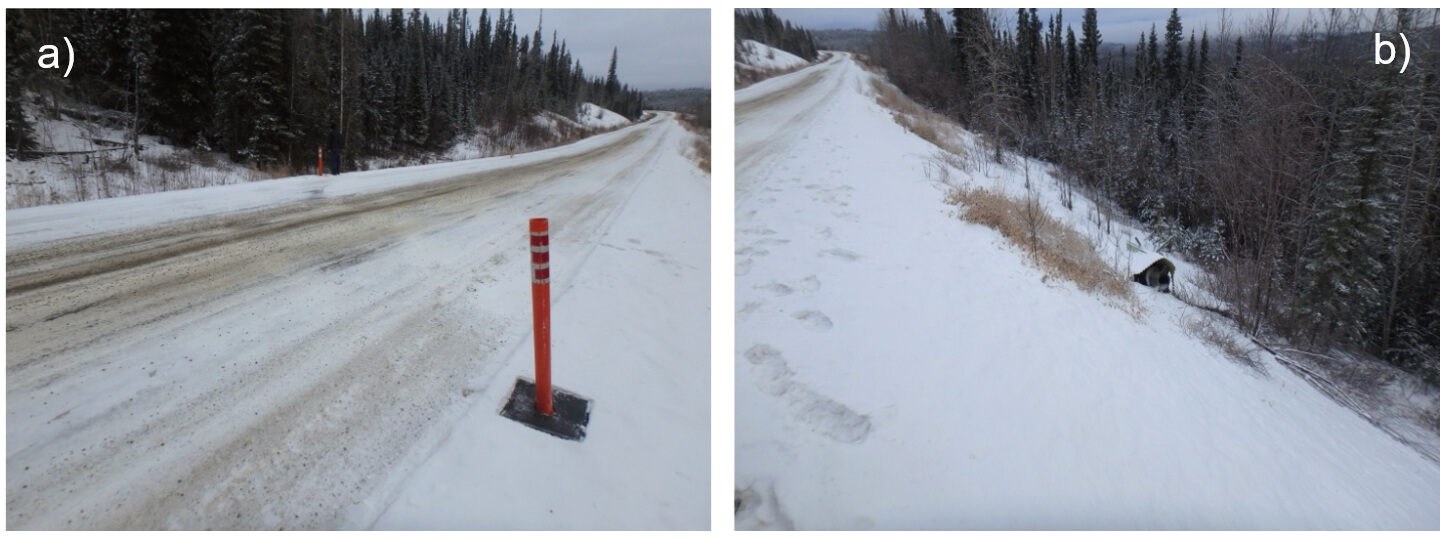
Borehole 10503-19 consists of coarse gravel near the surface grading into fine to medium gravel until 15 m. There is clay below 15 m to the end of the hole at 24.5 m. Resistivity values are between 100 and 350 ohm-m in the upper 15 m, going into 40 to 60 ohm-m below 15 m which indicates clay material. Figure 10 shows 2 photos from site 2 near borehole 10503-19. Photo a) shows a diagonal fracture running across the road with an approximate 5 cm elevation change. Photo b) shows the downside of the highway with a swampy area near the tree line.

Borehole 10503-16 consists of gravel until the end of the hole at 17.4 m. At a depth of 17.4 m a very hard substance was encountered which is interpreted to be hard bedrock. The gravelly material is wet, indicating no permafrost. The resistivity values are between 375 and 550 ohm-m with no change at 17.4 m depth. This is not surprising since gravel and the bedrock are both resistive with similar resistivity values.

Summary and conclusions

The RESOLVE survey provides a fast and efficient way to map the subsurface distribution of permafrost and to locate areas of frozen, partially frozen and unfrozen ground to depths of 100 m or more. The near surface resolution is approximately 5 m, approximately 10 m between depths of 10 and 50 m and increases to around 25 m at depths of 100 m or more. The resistivity depth slices and cross sections tie very well to the site 2 photo and the two deeper boreholes 10503-16 and 10503-19. Although not discussed, they tie to the site 1 photo as well. The sections and slices can be used to provide a regional overview of the area and can extrapolate point data such as boreholes to provide continuity between these localized centres. RESOLVE surveys, combined with high resolution digital elevation models, are also useful to monitor resistivity changes within the subsurface by flying the same areas at regular time intervals.