Seismic modelling of unconventional reservoirs

Introduction

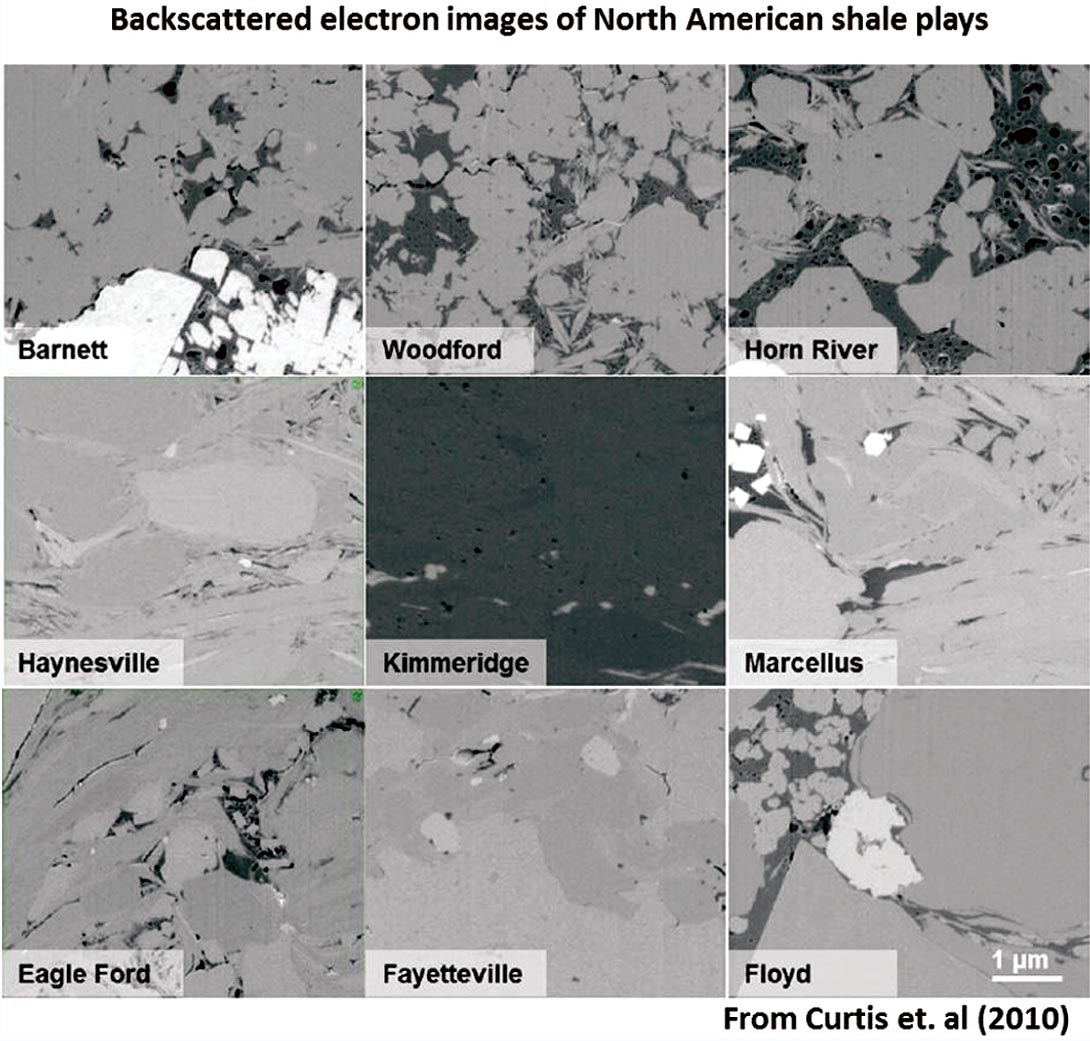
Unconventional resource development has become an exercise in determining where horizontal wells should be placed to maximize hydro-fracture efficiency. A large part of optimizing how the resource is developed requires understanding the reservoir from both lithologic and rock properties perspectives and correlating these with production data to infer frac efficiency. Given the variety of unconventional plays in North America, it is important to understand the differences in rock properties so as to effectively map them seismically. Figure 1 shows backscattered electron images displaying the diversity in microstructure beyond the differences in lithology.

Understanding the variations in terms of mineralogical composition and microstructure requires an in depth model. With such a model, templates can be generated for interpretation of seismic attributes.

The following is an examination of two distinct rock physics models and how they can be employed to generate seismic interpretation templates. These templates can then be used in conjunction with inverted volumes of seismic attributes to map lithologic and rock property variations. In addition, from the rock physics trends, AVO models are synthesized to evaluate potential offset dependent amplitude responses.

Two different rock physics models

The process begins with a comparison of two distinct rock physics models. Each model will be reviewed, referencing previous important works followed by suggesting potential application to unconventional reservoirs. The first is a granular model referred to as the modified Hertz-Mindlin Hashin-Shtrikman (HMHS) while the second, referred to as the Non-Interacting Approximation (NIA) is an inclusion based model which describes the number of pores and their shapes as opposed to the grain to grain contacts.

The modified Hertz-Mindlin Hashin-Shtrikman (HMHS)

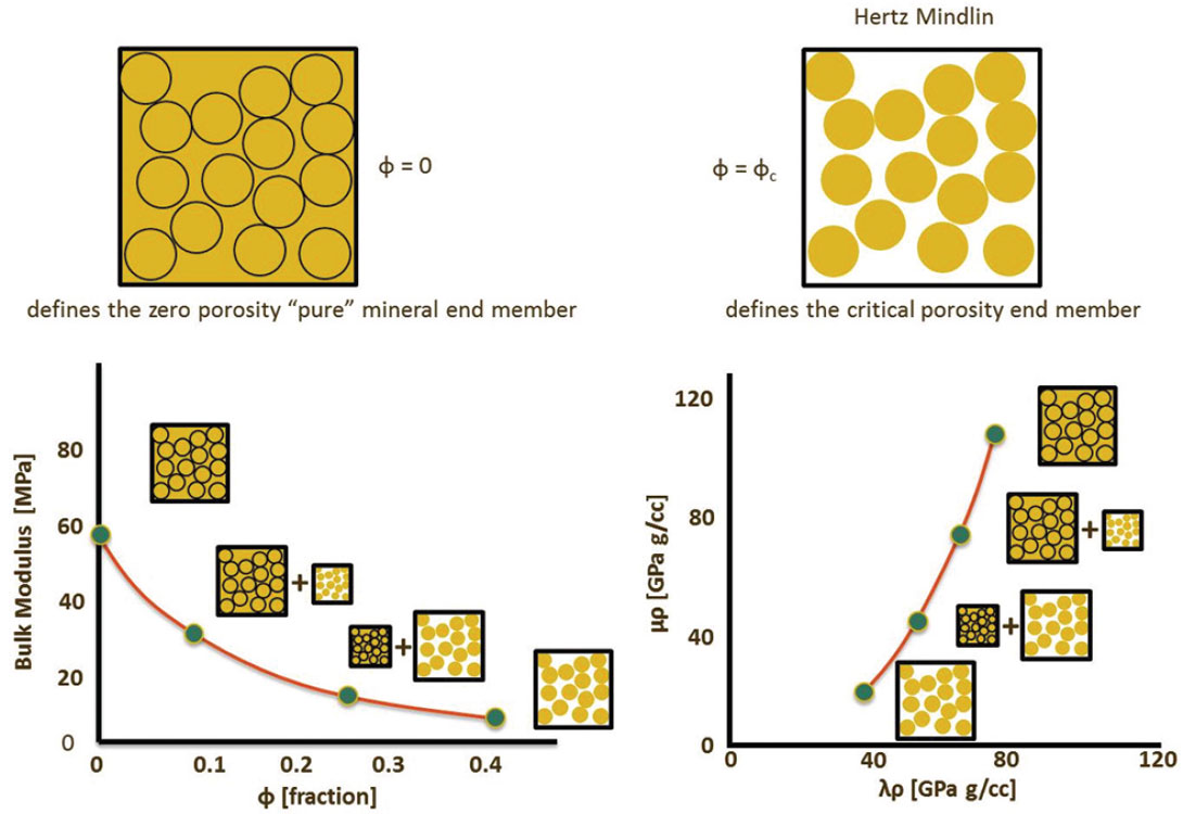
This model is a granular representation of a rock in that it assumes a random packing of spheres under hydrostatic compression. Contact between spheres is used to estimate bulk and shear moduli in terms of normal and tangential stiffness. The expressions for the dry bulk and shear moduli, known as the Hertz-Mindlin estimates, are given by (Dvorkin and Nur, 1996)

where n is the coordination number (number of grain contacts), φ is the amount of porosity, ξ is a grain frictional coefficient (more on this later), and R is the grain radius. The normal and tangential stiffnesses are

where G and v are the shear modulus and Poisson’s ratio of the sphere. The variable a is the radius of the contact area between the two spheres and an estimate is given by Hertz,1882 (Duffaut et. al, 2010),

where F_N is the confining force acting between the two spheres, given by

and P is the effective hydrostatic confining pressure.

The scalar value of ξ varies between 0 and 1 where 0 implies no friction between grains and 1 implies infinite friction. There are models that describe the variation of the parameter ξ. Duffaut et. al (2010) and Bachrach and Avseth (2008) studied the impact of the parameter and proposed non-linear and linear expressions, respectively, to model frictional variations. Bachrach and Avseth (2008) also investigate the effects of grain shape (round versus angular) with respect to the contact radius and its influence on the bulk and shear moduli.

The Hertz-Mindlin estimate of K and G is used to describe a rock at the critical porosity end member. This end member is assumed to represent the starting point of rock formation. Any porosity greater than the critical porosity will result in grains in suspension; not frame supported (Nur et. al, 1998). The Hashin- Shtrikman bounds are used to connect the critical porosity and the solid, zero porosity end member to create upper and lower limits for porosity values between the end members. This tren is schematically shown in figure 1, along with the associated LMR representation. These upper and lower bounds have been used to describe cementing and sorting trends (Avseth et. al, 2010).

The Hashin-Shtrikman bounds describe lower and upper limits to n-phase mixtures. The Hashin-Shtrikman bounds have the form (Mavko et. al, 2009)

where

where K_n and G_n are the bulk and shear moduli of each phase, fn is the fractional quantity of each phase and G is the maximum (upper bound) or minimum (lower bound) shear modulus of all the phases.

In the modified HMHS, which incorporates the critical porosity concept, the bounds consist of two phases (n=2): the Hertz- Mindlin defined critical porosity and the mineral, zero porosity end member.

The Non-Interacting Approximation (NIA)

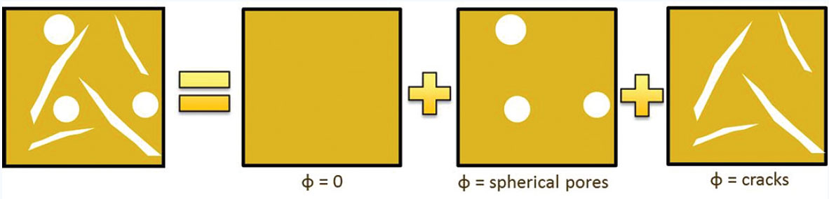
The second model, referred to as the non-interacting approximation (NIA), has been explored (Kachanov 1992, Kachanov et. al, 1994 and Shafiro and Kachanov, 1996) in great detail. This approach constructs the elastic potential of a solid with cavities (pores of various shapes including cracks) for both isotropic and anisotropic scenarios. The basic form of the NIA expression is a sum of individual compliances of components comprising the rock (Vernik and Kachanov 2010) and is illustrated in figure 3.

Note that the expression is linear in compliance and differs from Husdon’s approach in that Hudson deals with stiffness and has a linearization approximation.

The elastic potential is

where σ is stress and e is the strain. Hooke’s Law is invoked to describe the strain on the object as

where S^solid is the compliance of the solid material and Δe is the additional strain due to inclusions defined by

where S^incl is the so called cavity compliance tensor. For each cavity of interest, the cavity compliance tensor S^incl must be calculated. The total compliance of the material is the sum of the solid plus the cavity compliance for each pore shape being described. The elastic potential can then be expressed as

Once the equation has been set up with appropriate cavity compliance tensors for each pore shape, the moduli of interest can be determined from the stress strain relation. The compliance matrix S^ijkl can be of any form and is not exclusively appropriate for isotropic materials. In this instance, the analysis will be restricted to the isotropic scenarios (a subsequent paper will delve into the anisotropic models).

To account for the interaction between cavities, Kachanov proposes using Mori-Tanaka’s scheme (1973) where the average stress of the effective material is

The expression for σ_avg now replaces σ in equation 13.

As per Vernik and Kachanov (2010), a spherical pores and crack density expression would be

where v is the Poisson’s ratio of the solid, φ is porosity and n is the crack density. Note that:

1. there is no stress dependence in this expression
2. porosity affects cracks, but cracks do not affect porosity.

Model comparison

The following will be an examination of the two different rock physics models introduced. Specifically, the impact of pore shape as described by the NIA model is investigated in an attempt to rationalize differences between the granular and inclusion models. For the trends that follow, the rock is composed of 50% quartz, 25% clay and 25% limestone, representative of unconventional reservoirs.

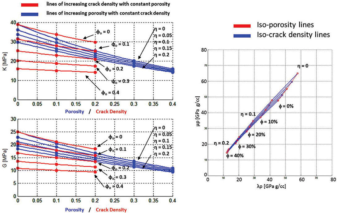
Figure 4 shows the differences between the granular model and inclusion model with spherical cavities. It is immediately apparent that the NIA model generates much larger values of bulk modulus (K) and shear modulus (G) for various amounts of porosity.

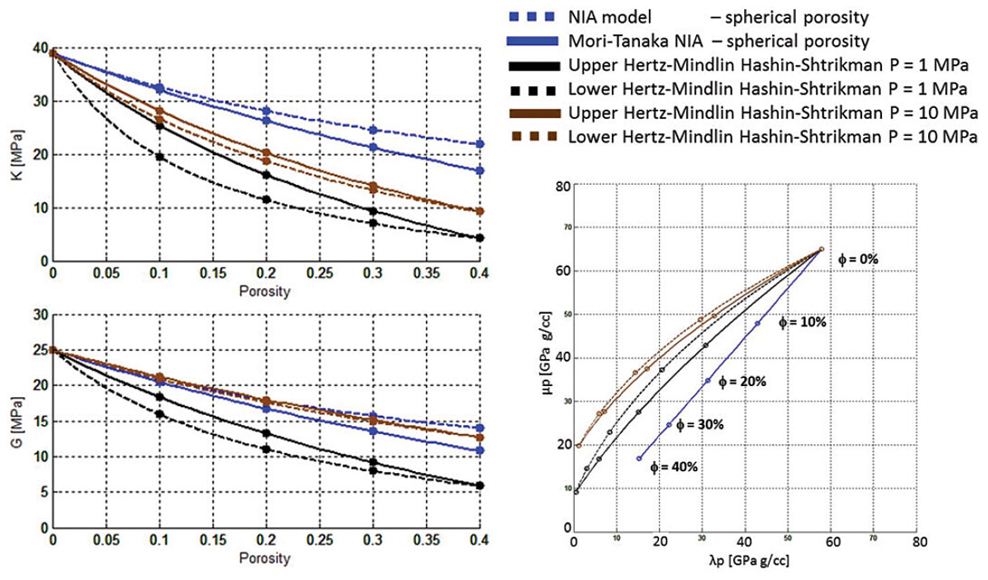
The blue dotted line overlies the solid blue line in LMR space. This means that the Vp/Vs ratio of the trend does not change by accounting for pore interactions; it is merely a change in porosity scale.

To rationalize differences between the models, an attempt to match the trends is made by adding pores of different shapes in the inclusion (NIA) model, shown in figure 5. The first attempt is the inclusion of infinitely thin cracks. The impact of cracks is to decrease K and G with increase in crack density, n. As in the previous figure, in addition to the K and G versus porosity / crack density plots, an LMR crossplot is included to demonstrate the expected response in a seismic attribute space. Note that at large porosities the effects of cracks is minimal.

The next pore shape shown in figure 6, is that of penny-shaped cracks. The impact is larger than in the infinitely thin cracks.

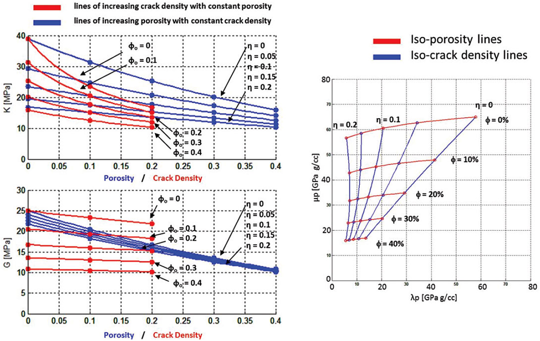
At first glance, it is observed that the appropriate pore shape and concentration could be constructed to mimic the granular trends. Though not demonstrated in the figures, it is postulated that the granular trends could be a representation of many different pore shapes ranging from spherical pores, penny-shaped cracks and thin cracks at high porosities, to just thin cracks at low porosities.

Fluid Effects

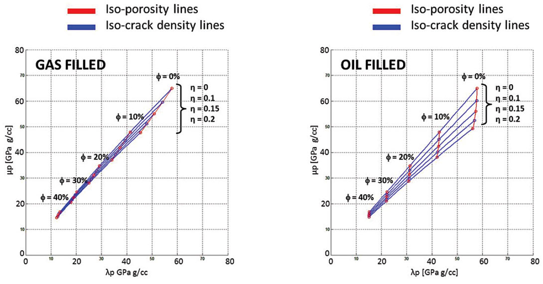
For fluid-filled pore spaces, Gassmann’s theory for fluid substitution (Smith, 2003) can be used to estimate the bulk and shear moduli for various amounts of porosity and fluids. Gassmann’s fluid substitution is suitable for the NIA and HSHM models (Grechka, 2007). The special case of fluid-filled cracks is shown to have a dependence on the crack aspect ratio as well as the fluid itself (Shafiro and Kachanov, 1997). Figure 7 above shows Gassmann’s results for gas and oil filled trends.

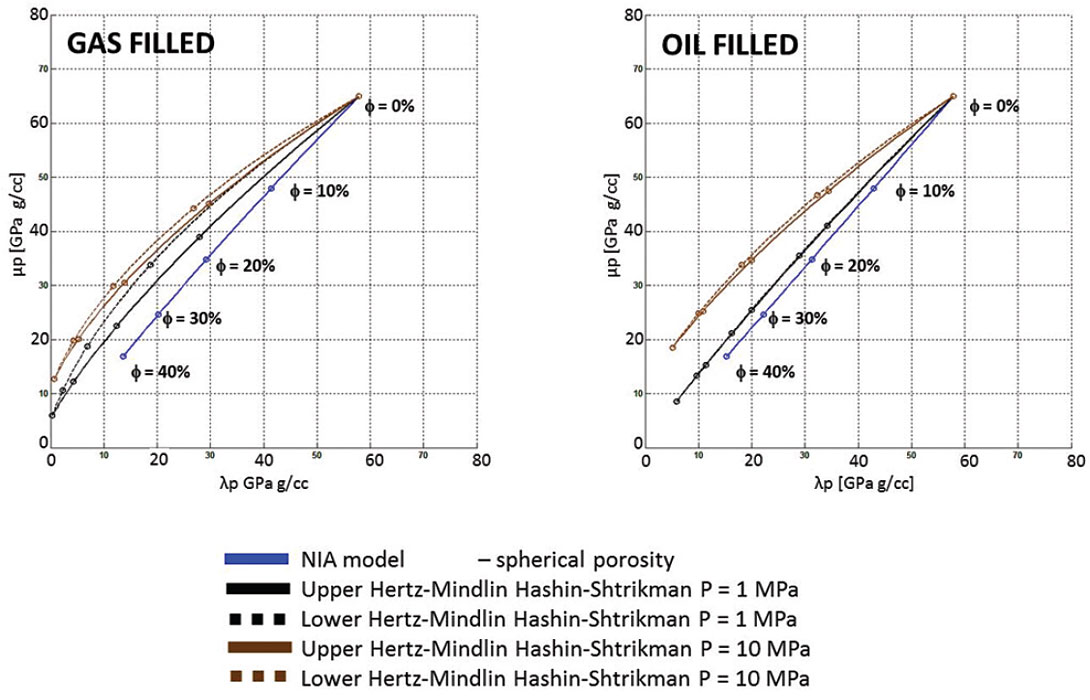
Note that the oil filled low pressure HMHS trends almost completely overly each other.

Figure 8 shows the inclusion based model (NIA) incorporating fluids and displaying some interesting results. Figure 8 shows the differences between gas and oil filled penny-shaped cracks (aspect ratio 0.1).

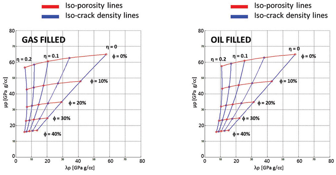
For thin cracks the response in LMR space is shown in figure 9.

The left figure shows the gas response while the right shows the oil response. Note that there is a slight increase in λρ as the cracks become filled with incompressible fluids. The presence of fluid strengthens the rock as seen from the parameter λ. The combination of figure 8 and 9 show the impact of crack aspect ratio in conjunction with the presence of fluids.

Multi-mineral models

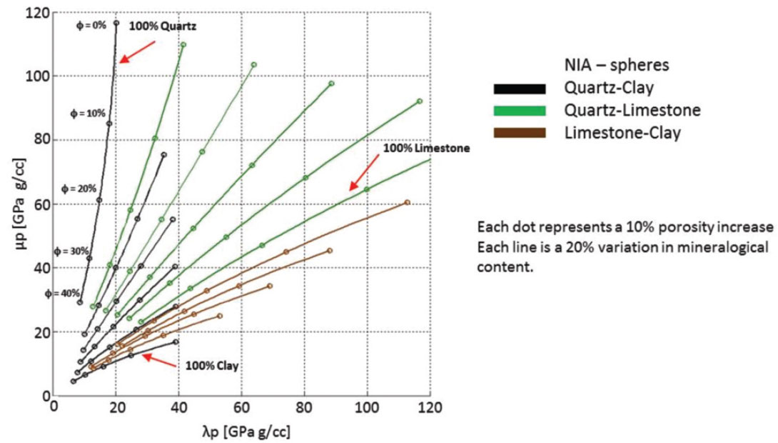
Potential unconventional templates can be modelled as a mixture of quartz, clay, and carbonate material, each with varying quantities. How to visualize the available permutations with the number of variables (mineralogy, fluid, porosity, pore shape, etc.) becomes a large part of the interpretation process. Comparing the previous LMR crossplots, there is overlap amongst the trends and thus ambiguity in the interpretation. One way to visualize the various lithologic permutations is to construct a two mineral trend demonstrating the variations in mineralogical composition and porosity. Figure 10 illustrates three such dual mineral trends: quartz-clay, quartz-limestone and limestone-clay.

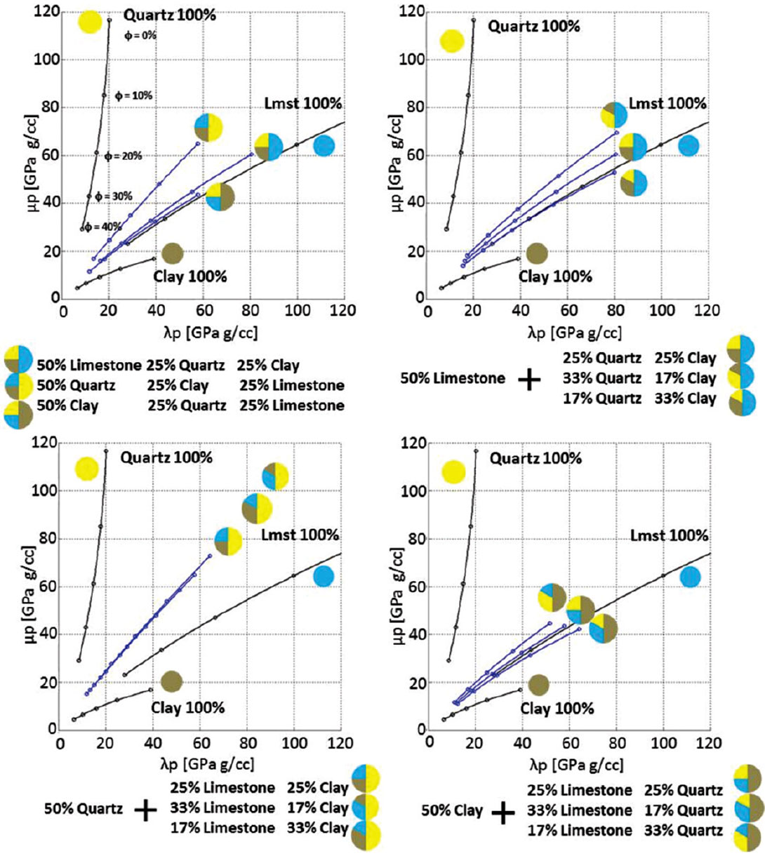
Another method could be to select three minerals and determine a distribution that would encompass the majority of potential outcomes. Figure 11 demonstrates the effects of a three mineral combination; quartz, clay and limestone.

Examples

Examples of well logs from three different unconventional resource plays in western Canada are presented with potential rock physics trends that can be used for interpretation. Each of the three examples will have a unique template in addition to a more generic multi-play template. The generic multi-play template is added to demonstrate the variability in each play with respect to a fixed template.

The importance of data integration cannot be overemphasized as using the templates in isolation would leave an interpreter with a myriad of possibilities that would minimize the predictive power of the trends. Without additional constraints, the use of modelled trends is not optimized.

Horn River

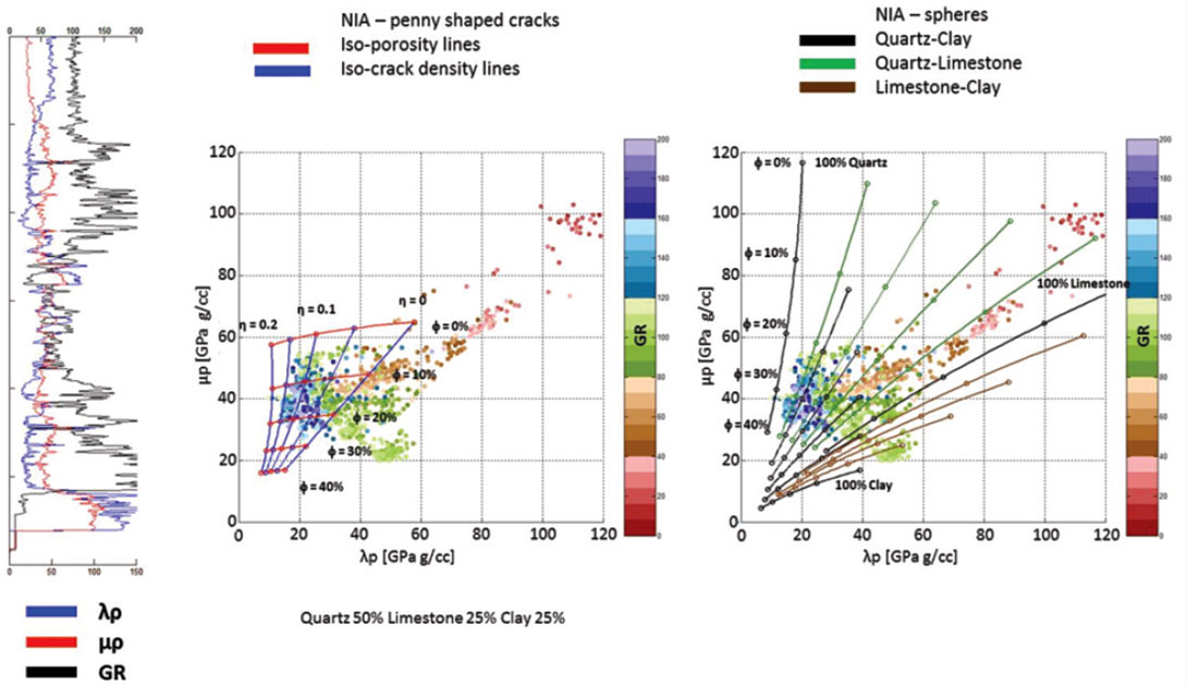
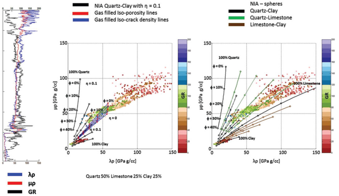
Figure 12 shows LMR and Gamma Ray (GR) logs along side two LMR crossplots each superimposed with two different rock physics interpretation templates.

The template on the left assumes a single mineralogical mix of 50% quartz, 25% limestone and 25% clay. The trends are generated using the NIA model. Each blue trend corresponds to increasing amount spherical porosity for a fixed penny-shaped crack density. The red trends correspond to increasing crack density for a fixed amount of spherical porosity. In this case, the LMR reservoir variations are attributed entirely to the concentration of penny-shaped cracks. Decreasing LR values are purely a function of increased crack density. Conversely, the crossplot on the right is the template introduced in figure 9. These NIA trends assume spherical pores and varying amounts of minerals. In this case the low LR values correspond to increasing quartz content. The “correct” interpretation template is likely a combination of these templates as well as other pore shape and mineral combinations.

Duvernay

Figure 13 shows LMR and GR logs for a Duvernay well, again with two LMR crossplot with two interpretation templates. The carbonate rich section (low GR data approaching 100% limestone trend) corresponds to overlying section.

It is noted that the Duvernay interval displays a more linear trend compared to the Horn River data. The log data also manifests itself in a range that can be suitably modeled by the quartz rich templates of figure 11. With that in mind, the blue trend lines correspond to an NIA model with a constant mineral mix of 50% quartz, 25% clay and 25% limestone, with increasing spherical porosity and a constant amount of gas-filled thin cracks. The black trend lines correspond to an NIA quartz-clay mix with increasing spherical porosity and a constant amount thin crack density. The crossplot on the right are the same trends shown in figure 11. Given the narrow range of Vp/Vs in the crossplot, one can make the assertion that this well contains very little lithologic variation (or has other minerals with similar bulk and shear moduli as quartz, clay or limestone) and any variations seen could be a function of pore shape.

Montney

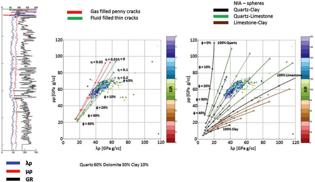
Figure 14 shows LMR and GR logs for a Montney well as well as set of two interpretation templates. Again, the right crossplot is the dual mineral mix introduced in figure 10. The crossplot on the left however, has NIA trends composed of 60% quartz, 30% dolomite and 10% clay with spherical porosity and various amounts of penny-shaped cracks. The red trends are gas-filled inclusions while the green trends are fluid-filled. Like the Duvernay, Montney rocks display a linear trend in LMR space, indicative of small Vp/Vs changes within the interval.

AVO Template Generation

The rock physics trends can also be used to generate a range of potential AVO responses that can be used to interpret seismic data without inverting the data. A large number of different scenarios can be modelled. Note that the four examples shown follow the expected behaviour as outlined in Perez 2010. Figure 15 shows the AVO responses expected from a clay rich layer overlying quartz, clay and limestone dominated layer. This may represent the transition from overlying non-reservoir shale to a potential unconventional reservoir. The ability to differentiate between quartz, clay or limestone dominated unconventional targets helps in understanding frac efficiency.

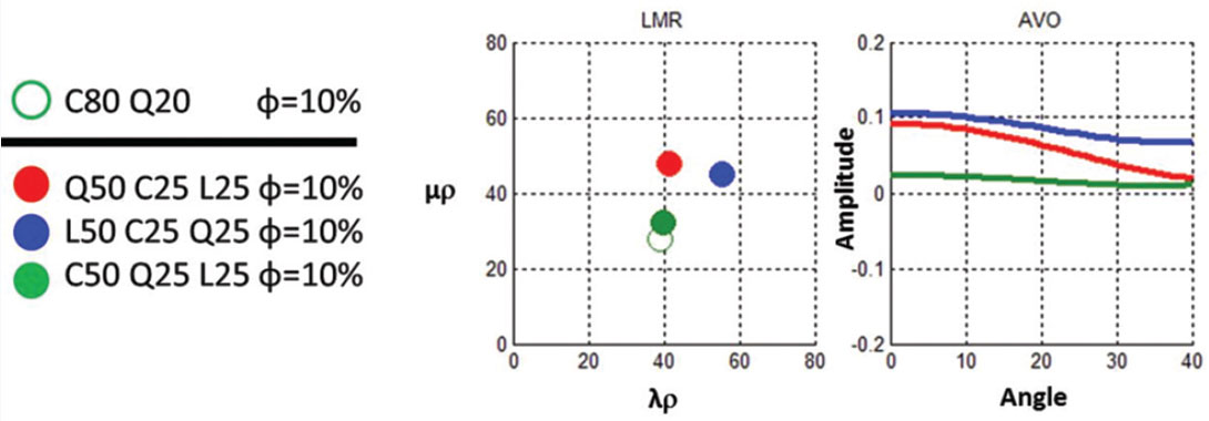
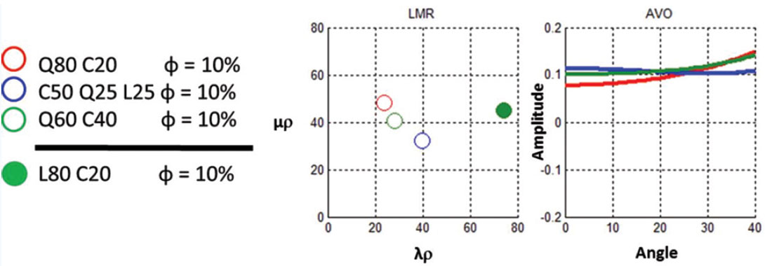
Figure 16 shows AVO and LMR plots of what could be representative of a transition from clay dominated to quartz or limestone dominated reservoir. As demonstrated by figure 10, the largest impact in both LMR and AVO signature is a function of quartz content. This could be representative of intra-Montney reflections and demonstrates the subtlety in mapping lithologic variations with AVO.

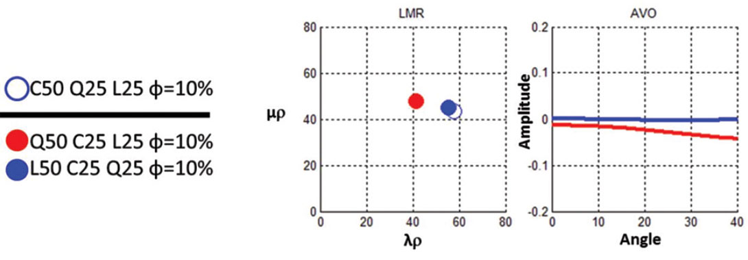
Figure 17 illustrates the effect of porosity and the ability of LMR and AVO signatures to detect such porosity variations. This shows a decreasing near offset amplitude and decreasing gradient with increasing porosity.

Figure 18 models the ability to detect potential carbonate rich frac barriers. In general, because the frac barrier is a “stronger” material, seismic expression is unsurprisingly a peak. The main control of the zero offset response is the high P-impedance while the lithology variations of the overlying layer control the gradient.

Two different rock physics models are introduced and used to interpret unconventional reservoirs from a seismic attribute perspective. The differences between the models are rationalized and potential interpretation templates are provided. Some AVO models are also generated demonstrating potential amplitude variations and the subtle nature of the seismic reflection in unconventional settings. These tools allow for a more in depth interpretation of seismic data.