The old and new in noise removal, wavefield representation and data regularization

Introduction

Traditional noise removal methods based on Fourier analysis, Radon transforms, and prediction filtering have occupied an important place in our arsenal of methods for noise attenuation. They all rely on different assumptions and, in general, on a simple signal model. An open problem in seismic data processing is the establishment of proper basis functions to represent seismic data. In addition, it is important to understand how one can use an optimal data representation to separate signal from random and coherent noise, and to regularize aliased and noisy data. We will review how old meets new and in particular, how one can complement well-known methods for noise attenuation with novel ideas in the field of sparse coding and compressive sensing. In addition, we provide examples of seismic data regularization where some of these ideas lead to algorithms amenable to regularizing data in the presence of strong coherent noise and aliased noise.

Local basis functions and sparsity

We start our discussion by considering the classical problem of representing a signal in terms of a superposition of basis functions. The representation can be written using the simple language of linear algebra as follows

where d is the Nx1 vector of spatial data and a denotes the Mx1 vector containing the coefficients of the expansion. The columns of the matrix G are the basis functions of the expansion. In general, this model is very flexible if we consider an overcomplete expansion. The latter, in simple terms, means that M>N. For over-complete expansions, we have an underdetermined problem and a priori information is needed to estimate the coefficients of the expansion. In real applications, equation (1) is further complicated by the presence of noise and incomplete sampling. This can be mathematically expressed via,

where n is the noise and T is a sampling operator. The underdetermined problem admits an infinite number of solutions. Among all possible solutions, we often chose one that leads to sparse representations (Olshausen and Field, 1996; Sacchi et. al, 1998; Hennenfent and Herrmann, 2006). The latter is a signal expansion where only a few columns of G are used to fit the observed data. We also stress that sparsity is the core of new paradigms in signal processing and harmonic analysis that are studied under the field of compressive sensing (Donoho, 2006).

The classical signal processing model maintains that a spatial signal must be sampled at a rate at least twice it highest wavenumber in order to properly represent the unrecorded continuous wave field. However, sub-Nyquist sampling is possible when the signal admits a sparse representation. This is known as compressive sensing or compressive sampling, a theory that has become quite popular in the signal and image processing communities (Candès a and Wakin, 2008).

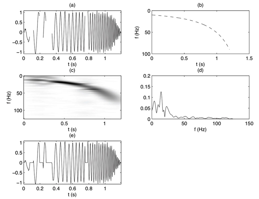
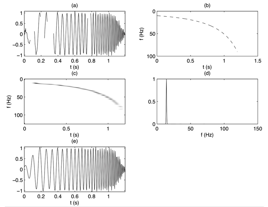
The importance of sparsity in data recovery problems can be demonstrated with a very simple example. Let’s consider basis functions given by Fourier complex exponentials that have been multiplied by a Gaussian window and translated in time. In other words, the expansion of the signal is in terms of Gabor atoms (Li and Ulrych, 1996). The coefficients of the expansion are a function of time and frequency or space and wavenumber. In Figures 1 and 2 we compare the reconstruction of a highly non-stationary signal using the classical Gabor expansion and the sparse Gabor representation. Figure 1a portrays a synthetic hyperbolic chirp with erasures. The instantaneous frequency used to generate the signal is portrayed in Figure 1b. The classical Gabor transform representation is provided in Figure 1c. In this case, one can show that the coefficients of the representation have minimum norm (in an L₂ sense). The reconstruction of the data is portrayed in Figure 1e. It is clear from these figures that the minimum norm solution to equation (2) has lead to coefficients that cannot recover the missing data. On the other hand, Figure 2 illustrates the case were sparsity was imposed upon the Gabor coefficients. Not only does the estimated Gabor t-f plane in Figure 2c shows fewer artefacts but, in addition, the Gabor synthesis was capable of recovering the missing samples.

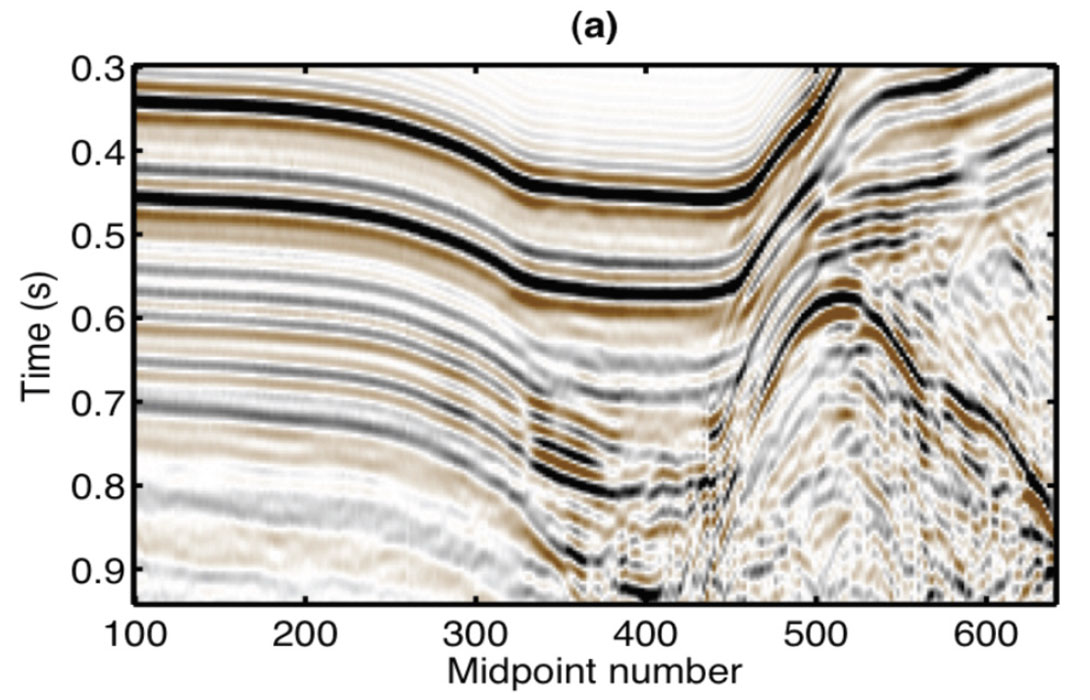
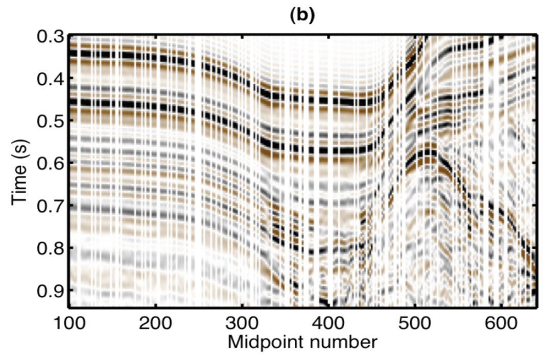
The aforedescribed algorithm can be modified to regularize 2D data with strong variations of dip (Sacchi et al., 2009). For this purpose, the reconstruction is conceived in the f-x domain where the 1D Gabor reconstruction algorithm is applied at each individual temporal frequency f. The results are shown in Figure 3.

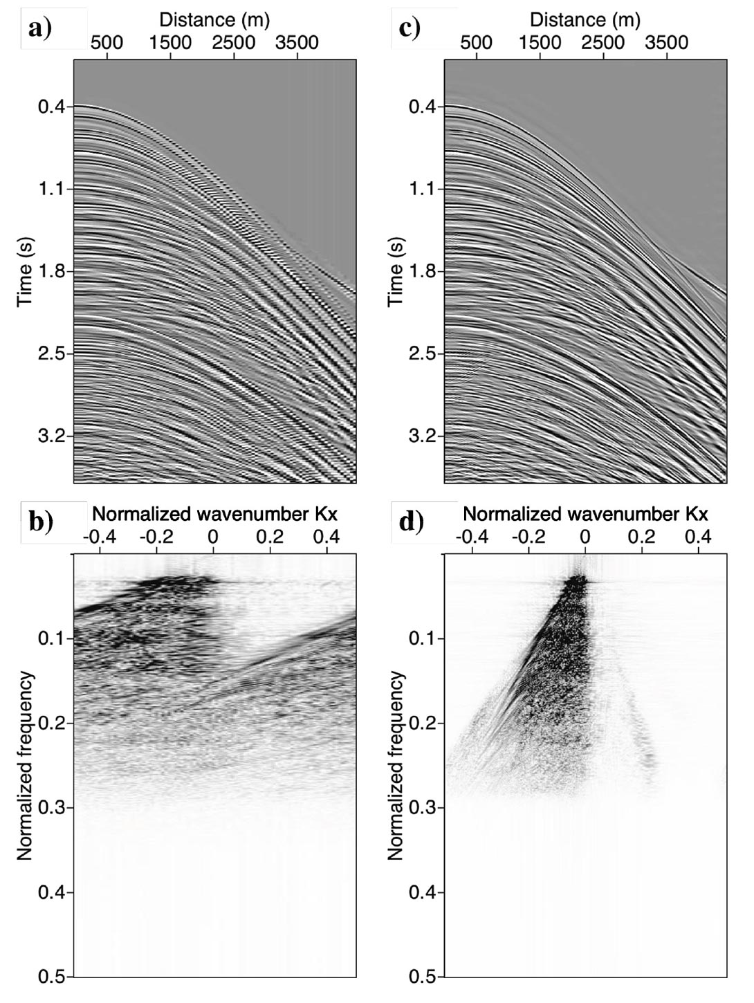
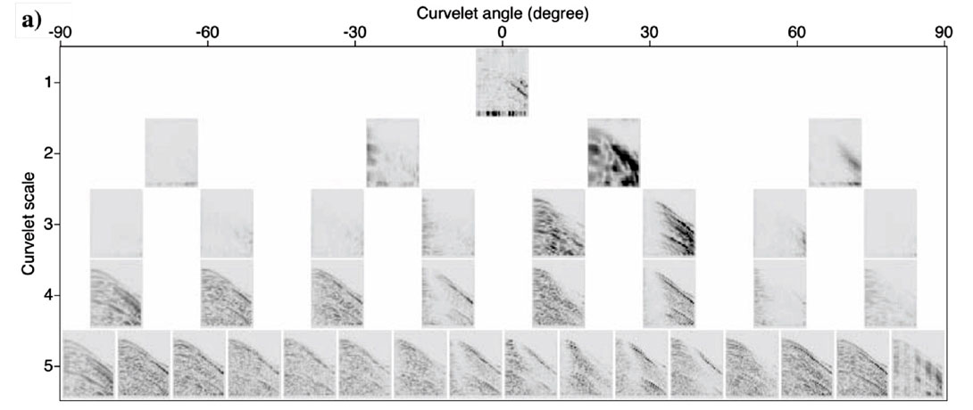
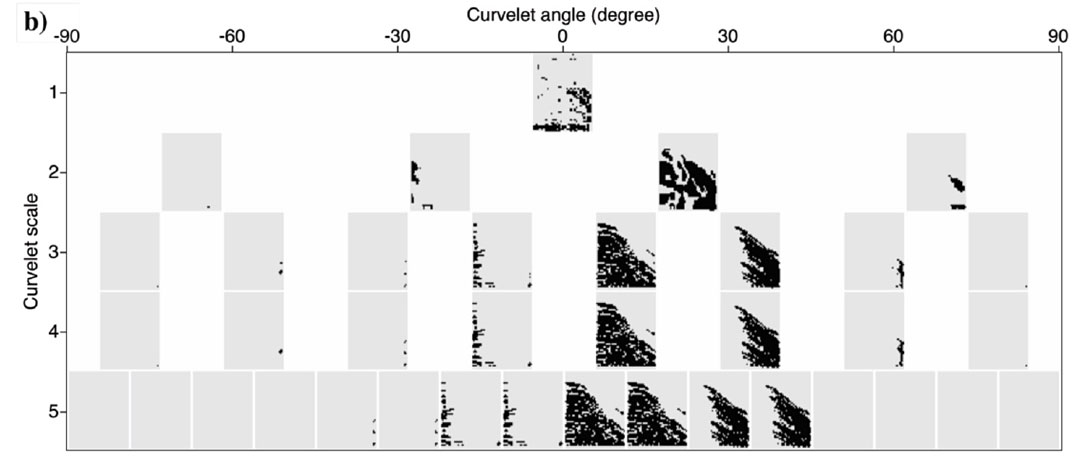
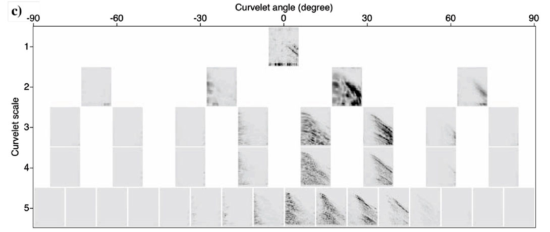
We now consider an example where the basis functions are curvelets. The curvelet transform is a local and directional decomposition of an image (data) into harmonic scales (Candes and Donoho, 2004; Hennenfent and Herrmann, 2006). The curvelet transform aims to find the contribution from each point of data in the t-x to isolated directional windows in the f-k domain. Figures 4a and 4c portray a shot gather before and after reconstruction using the curvelet expansion. It is well known that low frequencies are less likely to be contaminated by alias. This is clearly seen in Figure 5a where we have portrayed the curvelet coefficients in a diagram that shows the individual curvelet t-x patches organized according to scale (frequency) and directionality (angle or dip). Figure 5b shows a mask function derived by applying a threshold operator to the low scales. The alias-contaminated scales were annihilated using a mask function extracted from the low alias free scale (Naghizadeh and Sacchi, 2009). The mask function behaves like a local all-pass operator that eliminates the coefficients contaminated by alias. The surviving coefficients are fit to the observed data via the least-squares method. Finally, the estimated coefficients are used to synthesize the un-aliased data showed in Figure 4c. It is clear that this approach resembles the classical f-x (Spitz, 1991) interpolation method that relies on low frequency information to reconstruct aliased data. This is good example, we believe, of “old” ideas informing new development in signal processing.

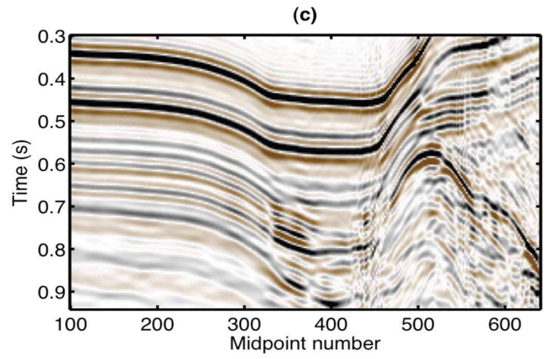
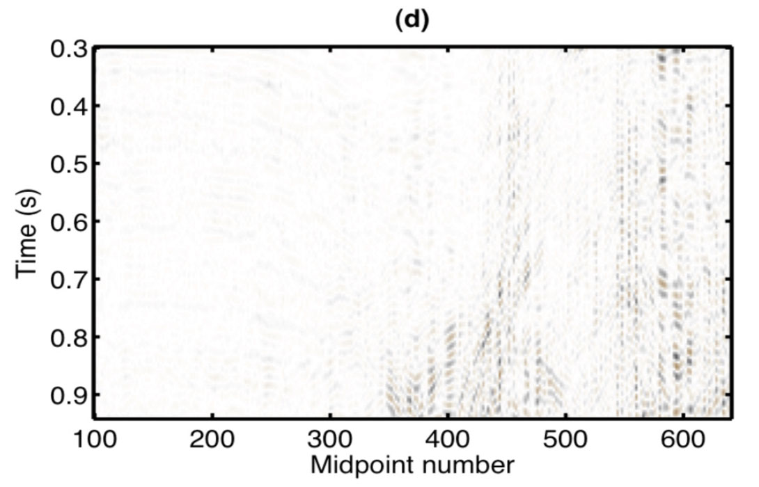
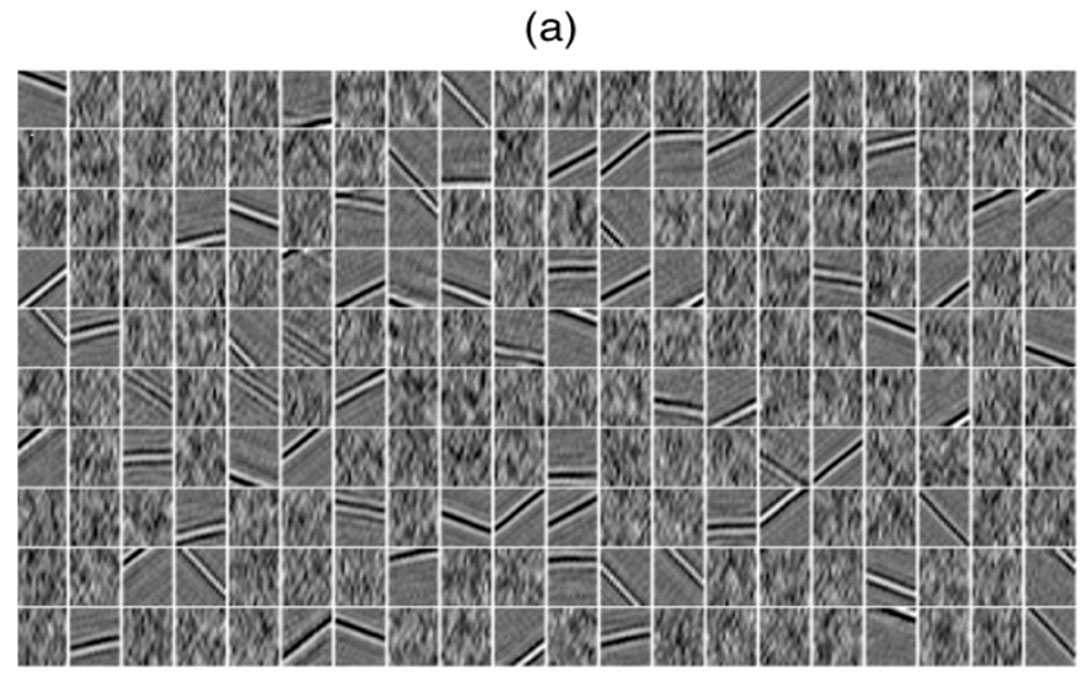
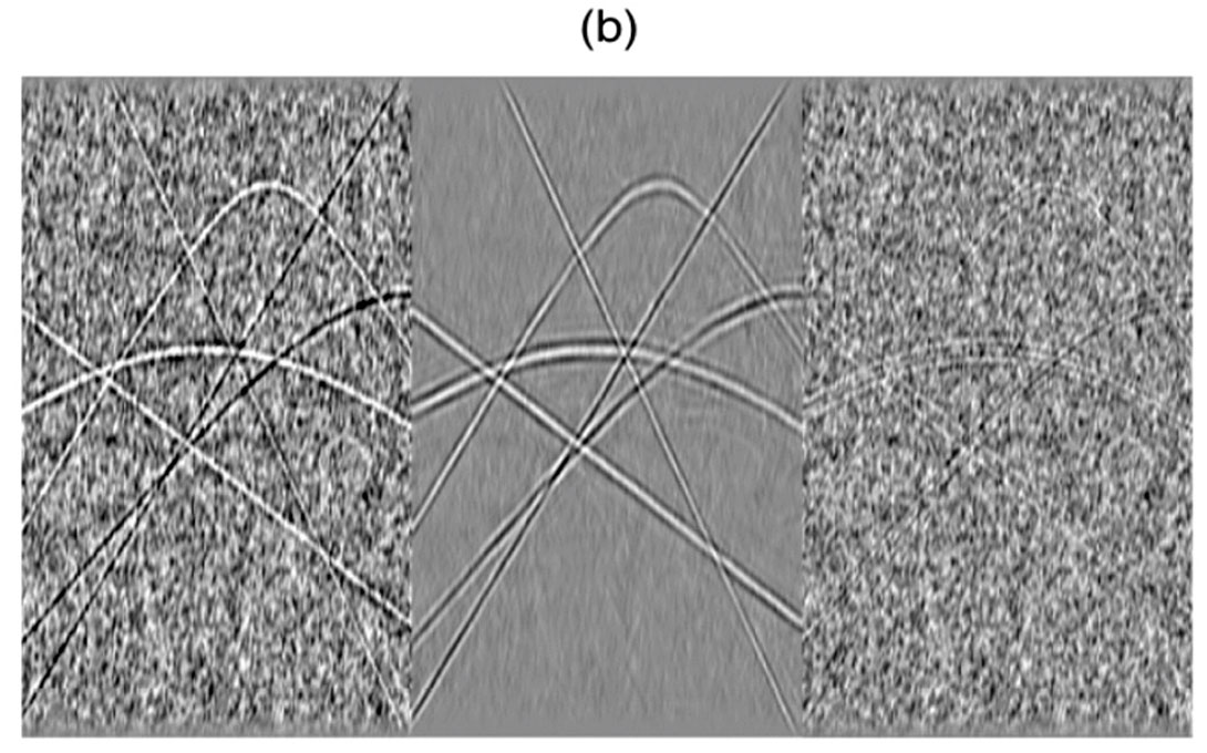
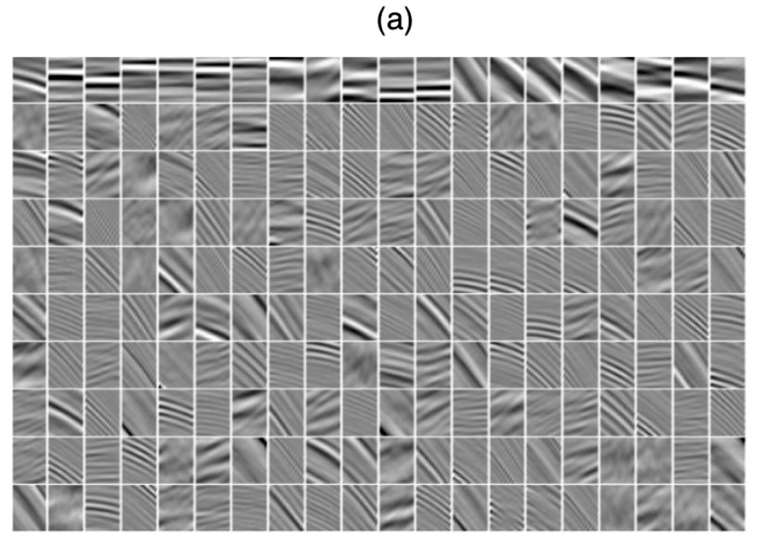
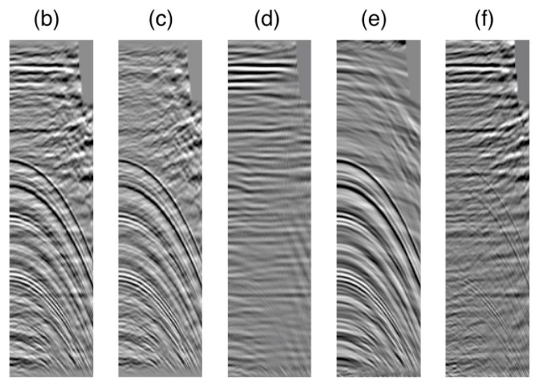
In our last example, we discuss the problem of finding an expansion of data by sparse coding. In this case, the basis functions are unknowns and are derived from the data. The problem is reminiscent of blind deconvolution where the reflectivity and the wavelet are simultaneously recovered from an observed seismic trace. Figure 6 portrays a synthetic example were the basis functions were extracted from the data via the algorithm described in Kaplan et al. (2009). The extracted basis functions were used to fit the data and the resulting de-noised image is provided in Figured 6b. The same method was used to isolate basis functions for the attenuation of multiple reflections. This is shown in Figure 7a. As we have already mentioned, the basis functions were extracted directly from the data. In this case, they were sorted according to smoothness and flatness, and those with the least amount of flatness were used to model the noise and the multiples. The model of multiples generated via the expansion with the retrieved basis functions is finally subtracted from the data to recover the primary reflections.

Conclusions

The concept of data expansion is fundamental for seismic data processing. We continuously represent our data in other domains and hope that these domains will help us to separate signal from noise, reconstruct data, and to analyze phenomena that are hidden in the original data space. The tools of linear algebra and linear inverse theory lead to interesting algorithms to retrieve sparse data representations that can be used for filtering, analysis and reconstruction.

We have briefly discussed the problem of estimating the basis functions from the data. The latter could lead to the new paradigms in seismic signal processing where basis functions for noise removal and for data reconstruction are estimated by exploiting data redundancy in seismic volumes.