Introduction
Hydraulic fracturing is known to generate seismic events, with magnitudes that typically range up to magnitude M0. The presence of these events has been widely exploited and interpreted in terms of fracture geometries and efficiency of stimulations. However, the reported magnitude ranges are dependent on the instrumentation used to capture the seismic data; the bandwidth of the instrumentation is tuned to a certain magnitude range, if events with magnitudes outside that range occur, then the reported magnitudes will be saturated. Only when instrumentation appropriate to the bandwidth of the events is used will the magnitude of the events be accurately captured.
Most hydraulic fractures are monitored with geophones with flat responses above 15 to 30 Hz, imposing a limit on the magnitudes that can be retrieved. In this paper, we discuss further this saturation effect and how deployment of an array of surface or near-surface sensors with differing bandwidths can be used to alleviate this effect.
Based on a case study, we discuss a surface array of 4.5 Hz and Force-Balanced Accelerometers (FBAs) monitoring the completion of a multi-well pad. Significantly large magnitude events were detected across this network, reaching magnitudes up to M2.9. Anecdotal reports indicate that the ground motion from these events was large enough to be felt on surface. The recorded waveforms corroborate these accounts with peak ground accelerations measured to be around 10 cm/s2.
Establishing the existence of these larger events occurring during hydraulic fractures is a significant result, and leads to questions on what conditions lead to the generation of such large events and what these events mean in terms the discrete fracture networks and overall production from the reservoir. We discuss how the source parameters of these large events give insight into these questions and how to properly contextualize the existence of such large events.
Characterizing Seismicity Across Many Different Magnitude Scales
Reports of large magnitude events with ground motions large enough to be felt during hydraulic fracturing operations have largely been restricted to anecdotal accounts. In cases where microseismic monitoring was employed to study the development of microseismicity during the completion, there has been a dearth of reports of large magnitude events as highlighted by Warpinski et al. (2012). However, using USArray network stations in Oklahoma, Holland (2011) suggests a connection between felt seismicity and hydraulic fracturing. Because the nearest stations in that study were 35 km away from the epicentres, uncertainties in locations were quite large and exact spatial relationships between the events and the injection wells were not well-resolved.
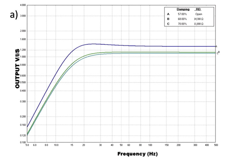
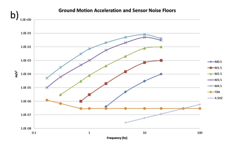
Aside from cases where signals are strong enough to be registered on national networks such as the USArray, most instrumentation used to monitor hydraulic fracturing is tuned to the magnitude range of the microseismicity, i.e. –M4 to –M1. Geophones, at their most basic level, consist of a damped mass-spring system, and as such have a natural frequency that is dependent on their components. To try to obtain a flat response over a wide band, shunt resistors can be employed, and properly configured will ensure a flat response from this resonant frequency to the frequencies that are typically well above the sampling rates. Figure 1a shows typical responses from downhole, 15 Hz, geophones with different levels of damping, featuring profiles that rise past the 15 Hz resonant frequency to a plateau where the instrument response should not impact the recorded signals. However, below the resonant frequency, signals will not be faithfully recorded. In comparison, the responses for 4.5 Hz and FBAs are shown in Figure 1b. For these sensors, the frequency response is above 4.5 Hz and 0.7 Hz respectively.
Because estimates of magnitude rely on the low-frequency response of the seismogram, the question of where the geophone resonant frequency is with respect to the spectral profile of the seismic event needs to be assessed before confident magnitude measurements can be made. Earthquakes are characterized by a displacement spectrum as shown in Figure 2: at low frequencies the displacement is relatively constant until a corner frequency at which point the spectrum decays at a rate proportional to the inverse square to inverse cube of frequency. The moment, and therefore the moment magnitude, is proportional to the amplitude of this low-frequency plateau. Other source parameters, like the radiated energy, the stress drop, the apparent stress, etc. depend both on the low-frequency plateau and the corner frequency. As discussed by Viegas et al., 2012, if this corner frequency falls outside the bandwidth of the instrumentation, then the source parameters calculated will depend on the instrument bandwidth rather than the actual response of the seismic event.
From Microseisms to Earthquakes: Seismic Responses Across Different Scales
As discussed above, Figure 2 shows that shape of a spectrum from a microseismic waveform. This shape of spectrum tends to hold regardless of event size, from the smallest microseisms to the largest and most energetic earthquakes. The similarity of response across several scales is evidence that seismicity generally behaves in a self-similar manner. That is that small events can be considered to be scaled down versions of large events.
From these profiles a number of different source parameters can be calculated (see Gibowicz and Kijko, 1994 for a review). For families of related events, a number of these parameters are relatively constant across a wide range of magnitudes. In particular, stress drop (the difference in stress before and after an event) and apparent stress (the amount of stress applied to the fault that is transferred into the radiation of seismic waves), can be constant for earthquakes in the same stress regime over a wide range of magnitudes. These parameters are usually inferred from other measures of earthquake source parameters, such as moment, and energy.
In the context of the triggering of large events, the constancy of the stress drop implies that the size of the fault ruptured, and therefore the moment magnitude of the event, does not necessarily depend on the triggering mechanism. In the case of a shearing event, the rupture process is resisted by asperities or barriers on the fault; when it encounters an asperity (a place where the two surfaces of the fault are locked) it will either grow past the asperity, into a large event, or stop due to the inability for the rupture to overcome the strength of the asperity. So the overall size of the event is not necessarily controlled by the stresses present. In areas where there are pre-existing fractures and faults present in the rock mass, this maximum size is controlled by the length scale of these structures; where large planar fault/fracture segments exist, stress perturbations in favourable orientations to the structural trend can lead to significantly large events.
The above discussion revolves around classical seismological concepts of triggering through the transfer of stress on favourably oriented faults. The role of injection induced pore pressure changes in general tends to move fractures and faults closer to failure. The role of pore pressure does alter some of the discussion on self-similarity, and variations in stress drop have been observed during injection processes with a good correlation to the expected perturbations in pore pressure around the injector (Goertz-Allmann et al., 2011). Notably, although the injection does change the stress settings for the failures, it will only assist the occurrence of larger magnitude events if the fluid manages to lubricate the faults present.
The activation of large structures could have potentially deleterious effects on the reservoir, if the seismicity represents the opening of a fracture that cross-cuts the formation allowing for fluid transfer into the cap rock or below. The relevant parameter in this case is the source radius, which will indicate the size scale of the fracture that has been activated. The source radius is determined from the corner frequency of the event with reference to models of the rupture process. For example, according to Brune (1970),

where rs is the source radius, β is the shear-wave velocity, fc is the corner frequency, and C is a constant of proportionality that depends on the exact model of the rupture process. The location, fracture orientation, and source radius will give the best indication whether the events will represent rupture into the reservoir, or not.
Case Study: Hydraulic Fracture Related Events Detected Locally and on National Networks
For this example, we document large events detected with a surface network of 4.5 Hz geophones and Force-Balanced Accelerometers. Two of these events reached magnitudes close to M3, and were strong enough to be seen on a regional seismic station around 100 km away from the treatment site. The regional network can only locate such events to accuracies of 10 km or better, which is insufficient to be able to distinguish whether such events are occurring on pad or off pad, let alone answer critical questions on the depth of the events (are they in zone, above zone, or below zone?) and other spatio-temporal relationships to the completion program. A local array of 4.5 Hz geophones and FBAs was in place, however, providing enough resolution to answer these questions. Furthermore, given the anecdotal reports of these events being felt on surface, the surface accelerations could be sufficient to begin to affect equipment on the frac site. In this case, it is necessary to gain a quantification of the peak ground accelerations that can be experienced.
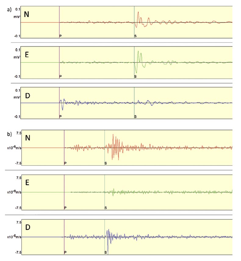
Two relatively large magnitude events occurred within close proximity of a hydraulic fracture completion on two consecutive days subsequently followed by hundreds of smaller events with M>0. The signals from these larger events are shown in Figure 3a from a relatively close-by broadband station (around 100 km from site). These signals were simultaneously recorded on a 5-station network of 4.5 Hz geophones and FBAs and the signal from one of these FBAs is shown in Figure 3b. Each station consists of three, three-component sensors deployed in a wellbore. Two 4.5 Hz phones are deployed at 25 m and 30 m depth, while the FBA sits closer to the surface at about 5m depth. The continuous data is sent from these phones to a central computer and are analyzed for potential triggers using an STA/LTA methodology, and then sent to an analyst for further interpretation.
The acceleration signals from the FBA and shown in Figure 3b for the largest events show peak values reaching about 10 cm/s2. The modified Mercalli scale (see Wald et al., 1999) relates these measures of the acceleration to the perceptions of people on the surface. The fact that this value for peak acceleration is observed lends credence to reports of these largest events being felt on surface, as these values for acceleration fall into the weak range that nevertheless should be felt.
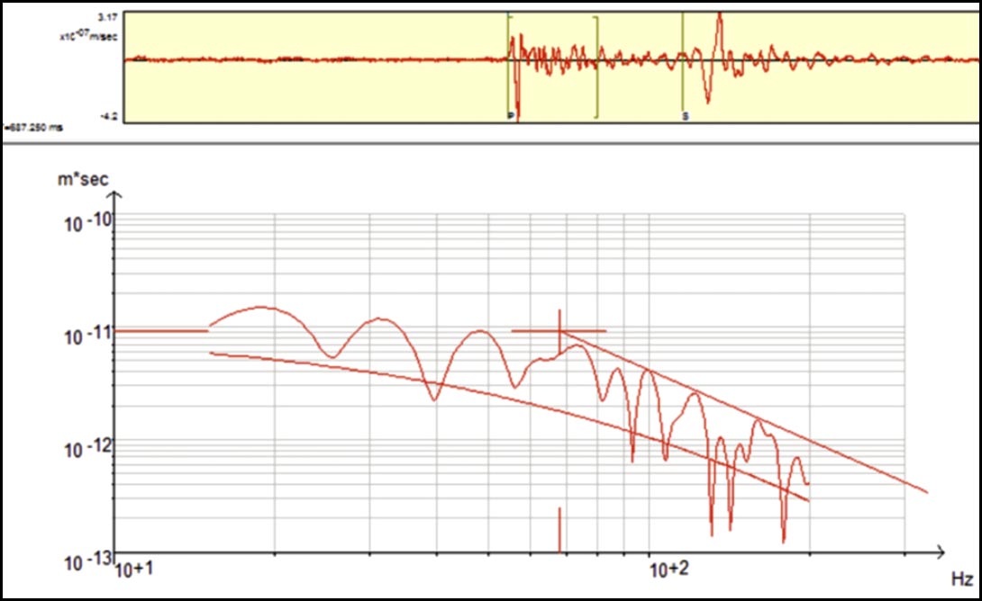
On the left of Figure 4, we show the spectrum of one of the largest magnitude event in the dataset as recorded on one of the FBAs. The corner frequency for this event is around 5 Hz and therefore the spectrum is only reliably recorded on the FBA. This estimate for the event corner frequency indicates that the size of the fault being activated is of a radius of 200m- 300m. Although events are locating below the treatment zone would suggest that they are being activated by stress transfer from the treatment, their dimensions (up to .4-.6km) suggest there could be fluid pathways between the reservoir and the surrounding formations.
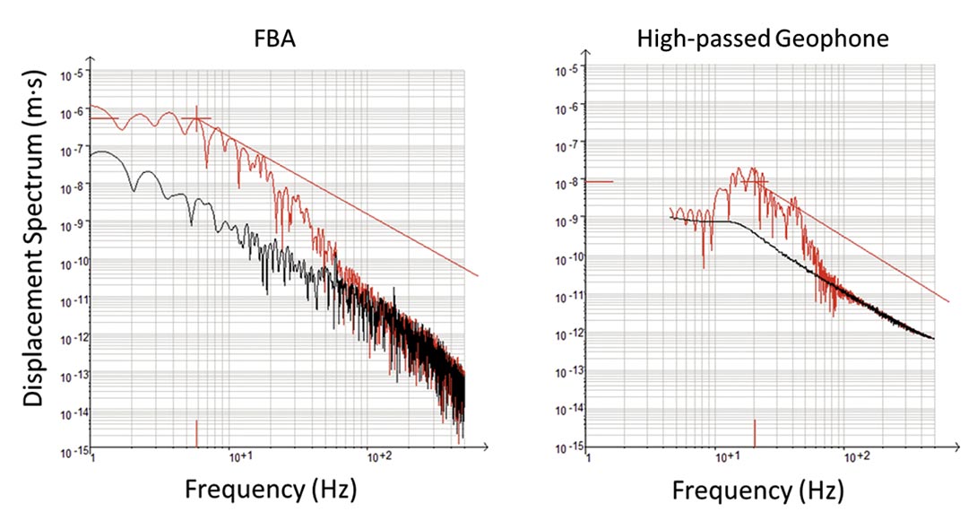
To illustrate the effect of magnitude saturation with a typical downhole geophone, we apply a highpass (15 Hz corner frequency) Butterworth filter to one of the 4.5 Hz geophone signals in the same well as the FBA highlighted on the left of Figure 4. Because the axes in both spectral plots are the same, one can immediately observe how much smaller the spectral plateau is for this signal plotted on the right of Figure 4. Therefore, without the lower-frequency component to the spectra, the magnitudes that are computed from the values of the low-frequency plateau of these signals will be completely underestimated. In this case, there is a full magnitude unit of underestimation observed for this signal. Perhaps more importantly, the signals in the time domain (above) are distorted relative to the clean discrete arrivals observed for the unfiltered low-frequency signals for the FBAs. One can conjecture that were signals observed in the time domain as in such events could be ignored as they would not be recognized as events that could be located.
As mentioned above, during the completion of the pad, not only were the two events at regional distances felt, but numerous other events were picked up by the local array with M>0. These events are depicted in plan view on the left of figure 5 with the well pad and surface stations shown for reference, and they are coloured by elapsed time and their size scale corresponds to their moment magnitudes. In order for a location to be determined, the event needs to be strong enough to be detected across the five stations. The colour scale reveals that these events are following the treatment program up the well to the heels over the days taken for the completion to be pumped. A depth view is shown on the right of Figure 5. These large events appear to be located beneath the wells and the target formations, suggesting the locations of the events tend to fall along two main trends, the early events follow a trend roughly 30° from SHmax and the later events follow a lineation approximately parallel to SHmax. In addition, there is another cluster of events, spatially located between the two linear distributions. The distribution of the first cluster of events is optimally oriented to slip given the direction of SHmax. The second linear cluster is in good agreement with the expected event trend, if the regional stress were controlling the overall event distribution. Furthermore, the trend of these locations with time is following the treatment program, earliest events are towards the toes of the wells, and the events drift towards the heels with time, reflecting the completion.
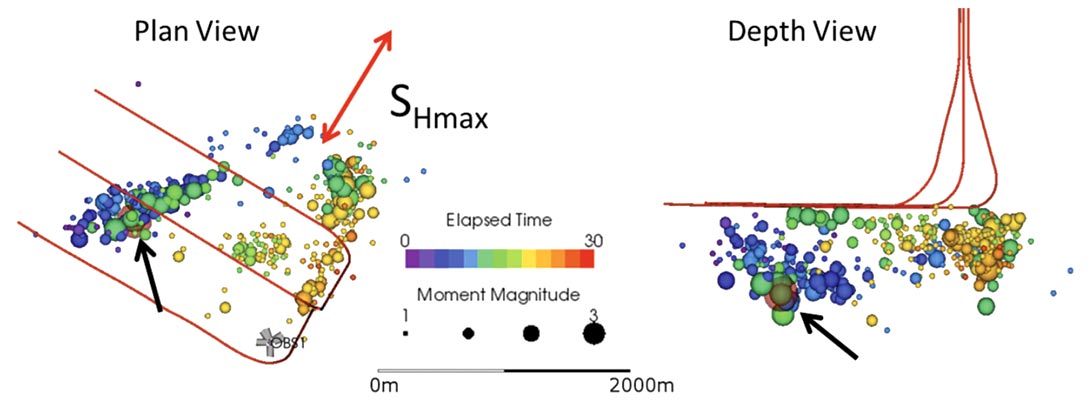 t distribution over the pad where the events are coloured by elapsed time and the size scale corresponds to moment magnitude. There is a black arrow in both views pointing to the event shown in Figure 3. One of the five observation stations is depicted in the plan view and the direction of SHmax is also noted. The treatment wells are displayed in red.
Discussion
We have detailed an example of relatively large magnitude seismicity begin associated with hydraulic fracture operations. For the example discussed, we hypothesize that the large events observed are activating larger, fault-scale features beneath the treatment formation that are optimally oriented to slip in the stress field in which the events are occurring. The recorded waveform peak values are in accord with the reports of these events being felt on surface. The recognition that events generated during hydraulic fractures can have the potential to be felt on surface is important for a number of reasons. From a perspective of due diligence, such events need to be as accurately characterized in terms of location and source parameters as possible (including magnitudes, but also source radii). The public concern about connections from the treatment zone to groundwater aquifers can be answered with these data. From the perspective of fault activation, often this is an undesirable consequence of hydraulic stimulation if these faults provide pathways for fluid to escape formation. Again, being able to position these faults with respect to the reservoir stimulation is of prime concern. Finally, if these events are generating ground motions large enough to be felt on surface, then there needs to be an assessment of the seismic hazard on site to answer questions about where shaking may be most intense and to what standards equipment needs to be built to withstand such motion.

Related Reading


Join the Conversation
Interested in starting, or contributing to a conversation about an article or issue of the RECORDER? Join our CSEG LinkedIn Group.
Share This Article