What Does Microseismic Tell Us About Hydraulic Fracture Deformation

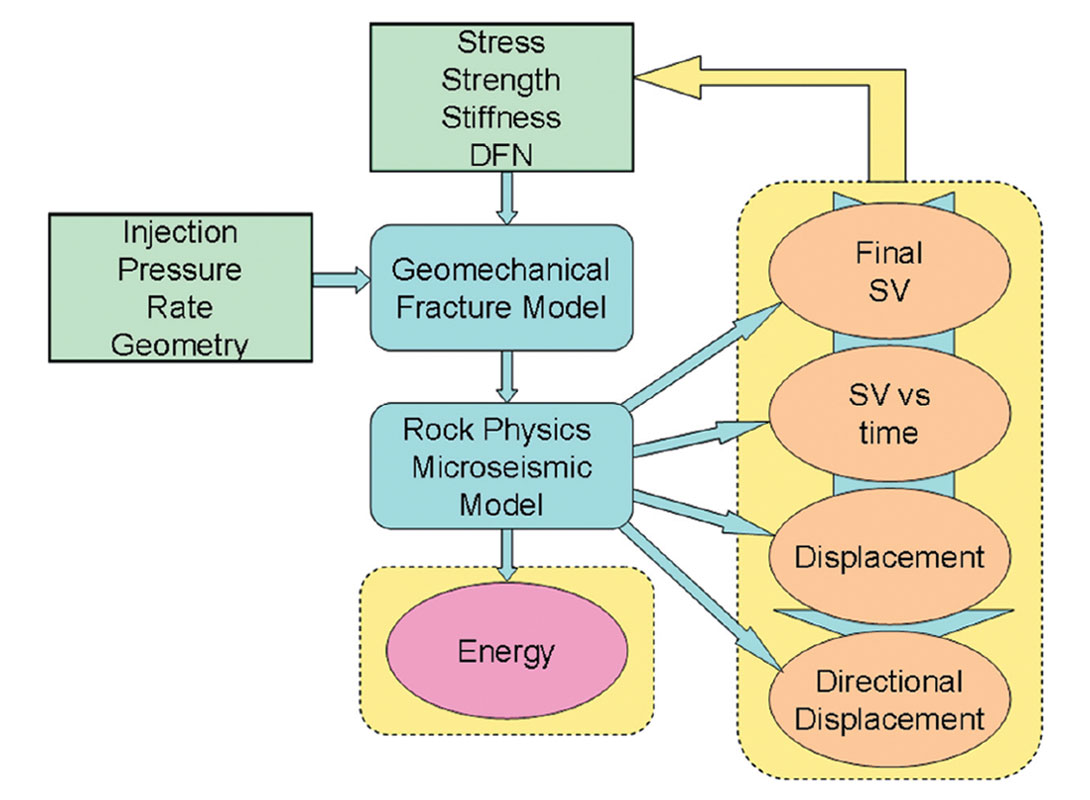
Introduction

With the expansion of microseismic imaging of hydraulic fracture stimulations in the past few years, interest has evolved from simply the event locations to extracting more information from the signals through advanced source characterization. Details about the fracturing and deformation associated with the microseismic source can be investigated using earthquake seismology methods and could potentially unlock further details about the hydraulic fracture process. Over the past few decades, the more mature mining and geotechnical applications of microseismicity have already witnessed similar evolutions from locations to advanced source characterizations, in each case ultimately resulting in recognition of the need for a geomechanical model to reconcile the microseismic with the overall deformation. In this paper, various aspects of the microseismic deformation are discussed in order to define how much we can say about the hydraulic fracture directly from the microseismic. A general geomechanical workflow is also introduced, which includes a rock physics model relating the microseismic portion of the deformation and enables a calibration and validation of a geomechanical model of the total hydraulic fracture deformation. Armed with this validated geomechanical model, ‘what if’ scenarios can be explored to provide engineers with a tool to optimize both the hydraulic fracture stimulation and the ultimate production from unconventional reservoirs.

Microseismic hydraulic fracture images are typically used to interpret fracture direction and dimensions, as well as the stimulated volume created during the treatment (Maxwell et al., 2002). Microseismic has become the dominant far-field fracture mapping technique and has lead to the development of a number of value added engineering applications. King (2010) presents a comprehensive review, including real-time fracture control to avoid geohazards and improve stimulation coverage along the well, optimizing completion design by improved staging and isolation, and improving field developments through strategic well placements and spacing.

Although most microseismic applications are related to determining fracture geometry, there is also the possibility to examine other source characteristics of the microseismic events (microearthquakes), using analysis methods developed for tectonic earthquake studies (see Gibowicz and Kijko, 1994 for a comprehensive review). Microseismic activity is generated by instantaneous geomechanical strain or slip and the microseismic source characterization provides details of the deformation or slip resulting in the microseismicity. The source characterization thus provides a snapshot of the geomechanical strain generating the microseismicity and hence details of the hydraulic fracture process. The most common microseismic source characteristic is the magnitude or strength of the microseismic sources (Maxwell et al., 2002). Magnitude has been used to examine detection limits for a given data set, identify fault interaction with the hydraulic fracture, and to improve stimulated volume estimates (e.g., Maxwell et al., 2006). A somewhat less common analysis method uses differences in the polarization and radiation characteristics of the seismic waves, and has been used to interpret changes in the microseismic source mechanisms (e.g. Rutledge et al., 2004, Maxwell et al., 2007).

Further source characterization can help understand the mechanics associated with the seismic deformation occurring during the fracture slip resulting in the microseismic signals (see Gibowicz and Kijko, 1994 for a comprehensive explanation of source characterization). Characterizing the microseismic source can take the form of source attributes computed by applying kinematic fracturing models to deduce the stress changed resulting from the seismic strain, and amount and area of slip. These methods involve modeling the seismic slip to match the observed seismic pulses using amplitude and frequency/time duration to estimate source strength, slip area and stress release. Another form of analysis involves seismic source mechanism studies, which examine the seismic radiation characteristics in different directions and attempt to define the fracture plane orientation and if the deformation is shearing and/or opening or closing. The most general source mechanism investigation uses a method called seismic moment tensor inversion, where the source strain tensor is estimated. Both source attributes and mechanism studies often use techniques developed in earthquake seismology to characterize shear deformations and lead to a common mechanism approach that is the so-called beach ball displays of seismic radiation from a shear deformation source. All of these earthquake techniques have slowly begun to be applied to hydraulic fracture monitoring, in attempts to gain insight into the fractures beyond simply mapping far-field geometry. It is naturally attractive to also use not just the location and timing but all aspects of the microseismic data to help understand the hydraulic fracturing process and potential effectiveness.

One of the main challenges applying these earthquake seismology methods to microseismic monitoring of hydraulic fracture treatments is the common use of a seismic array in a single monitoring well, which limits the directionality of the seismic radiation leading to uncertainty in the source investigations. A greater challenge, however, is that while microseismic source characterization holds promise to quantify how the microseismic fracture is deforming, there is a lack of a definitive rock physics model to provide context to interpret the underlying hydraulic fracture deformation response. In other words, in order to utilize the geomechanical strain of the microseismicity, we need to understand how it relates to the overall geomechanics of the hydraulic fracturing. Fracture engineering has been challenged for several years to be able to simulate the fracture mechanics of complex hydraulic fractures illuminated by microseismic monitoring of reservoirs such as the Barnett Shale, which suggests that the geomechanics is also a complex issue (Cipolla et al., 2008a). Microseismic provides an important and unique piece of this complex geomechanical puzzle.

Hydraulic Fracture Geomechanical Deformation

In the following section, various aspects of the deformation associated with microseismic events and the underlying hydraulic fracture are presented and contrasted. The relationship between these two aspects is relevant to the rock physics and geomechanics of the deformations associated with the microseismic and total fracturing of the rockmass. In the following discussion, the mechanics, rate and energy of the hydraulic fracture and microseismic will be compared. For context, the reader may find it useful to contrast these discussions with a traditional geophysical seismic source such as a vibrator, which is specifically engineered to provide consistent characteristics with the desired seismic waves. Vibrator sweeps are designed to maximize power within the seismic bandwidth, and the mechanical vibrations are designed to maximize coupling to efficient create seismic waves in the subsurface. In the case of hydraulic fracturing, however, the microseismic waves are indirectly generated by the high pressure injection to stimulate flow into the well. This comparison with a traditional seismic source will be further discussed later in the paper.

Hydraulic Fracture Deformation Mechanisms

The conventional view of a hydraulic fracture treatment is that as the injection pressure is raised to the breakdown pressure, the rock breaks or parts in tension resulting in increased injectability (e.g. Smith and Shylaporbersky, 2000). As volume is continued to be injected into the fracture the fracture grows outwards and also the fracture continues to open at a rate depending on the net pressure and fluid leakoff. Alternative views include the rock breaking under shear or a hybrid shear-tensile fracture, although such models seem to be an attempt to reconcile perceived microseismic mechanisms. Shear slip can result in enhanced permeability, as slip tends to result in fracture dilation resulting from topography differences in the contacting fracture surfaces (e.g. Barton, 2008). Nevertheless, the large volumes and long injection times of typical stimulations likely result in significant fracture dilation or opening in order to accommodate these large injection volumes (Daniel and White, 1980). Fracture width is also needed to accommodate proppant into the fracture. Therefore, even if shearing is a relevant mechanism for fracture creation, eventually opening modes must occur. If the shearing fractures evolve to opening modes during the treatment, the normal clamping force must relax which would reduce fracture strength and result in lower intensity of shear slip. In addition to such global views of the hydraulic fracturing, localized interaction or growth near or through pre-existing fractures could result in similar shearing and opening mechanisms. Nevertheless, tensile fracture opening is considered here to be the predominant mechanism of hydraulic fracture propagation. Similarly, pressure relaxation after the end of the injection will result in predominant fracture closing of the hydraulic fracture.

Microseismic Deformation Mechanisms

Early papers on hydraulic fracture induced microseismicity argued for a shearing type mechanism based on observations of relatively strong s-wave amplitudes (Warpinski et al., 2004). Indeed, strong s-wave amplitudes are diagnostic of a shear mechanism source. Moment tensor inversion studies model the seismic source strain tensor that results in observed seismic amplitudes by examining the source type and subsequent transmission to the seismic receiver, and enable analysis of the type of source: be it shear, tensile opening or closing, or explosion. While many examples show shearing, some recent studies report variable microseismic source mechanisms during hydraulic fracturing ranging from shear to tensile failures and also including components in between (Baig and Urbancic, 2010). The primary hydraulic fracture tensile opening mode could result in a microseismic source with a tensile mechanism, if the tensile parting results in sufficient slip in the characteristic time period of microseismic data (discussed below). If the rock is able to deform and strain under tension prior to failure, an instantaneous microseismic tensile source could occur. However, most reservoir rocks are unlikely to be sufficiently strong in tension/cohesion, to produce sufficient seismic energy to result in detectable microseismicity in a tensile failure mode. After the initial tensile failure occurs further tensile microseismic deformation would not be expected as the rock would slowly deform due to the increase of net pressure in the fracture. Since the rock has already failed under tension, it is also relatively weak and unable to store sufficient strain for continued generation of microseismic events in the failed region. Microseismic events associated with fracture closure are also possible from a seismologic point of view, although mechanically the phenomena is hard to rationalize especially during a hydraulic fracture injection since the pressurized fluid that mechanically dilates fractures will also tend to resist instantaneous (i.e. microseismic source time periods) closure. A physical analogy would be trying to clap your hands together underwater.

Mechanisms may be expected to vary between monitoring projects, depending on the local pre-existing fractures and stress state along with other factors in the mechanics of the microseismic deformation. Furthermore, there are many geophysical parameters that control observed seismic amplitudes/radiation patterns, and result in uncertainties in the derived moment tensor (e.g. Sileny, 2009). Local borehole anomalies near the sensors, seismic attenuation, energy partitioning with reflection of seismic waves, multiple phases and background noise can all impact the observed amplitudes and potential confidence in the moment tensor inversion. Uncertainties in any these factors can lead to uncertainty in modeling the wave transmission part of the analysis, and thereby impact the estimated moment tensor. Furthermore, uncertainties in seismic velocity or impedance models result in uncertainty in the transmission as well as potential accuracy of estimated source location, again leading to uncertainty in source type (e.g. Kim, 2011). Finally limitations in the angular coverage of seismic amplitude measurements due to limited number of observation wells leads to lack of uniqueness or ambiguity and an under constrained moment tensor inversion. Nevertheless, if accurately determined microseismic moment tensor is the most complete description of the source strain and provides key information about how the rock breaks to form microseismicity.

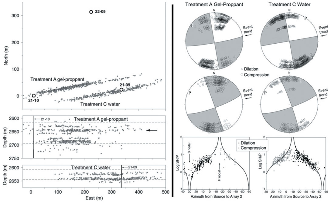
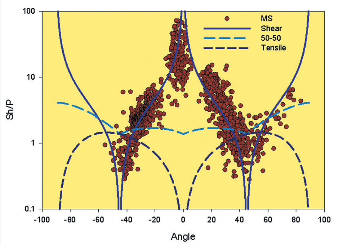
Rutledge et al., 2004, analyzed mechanisms of microseismicity recorded during hydraulic fracturing of the Cotton Valley sands (Figure 1), and in addition to composite beach-ball shear-type mechanisms, modeled sh/p amplitude ratios with a strike-slip, shear model. The composite solutions assumed a single source type for all events, and sample the radiation pattern through variations in the source-receivers angles. The strike-slip shear mechanism seems plausible since the model provided a reasonable fit to the observations. Note that these methods suffer an ambiguity between two possible slip planes orthogonal to each other, since the radiation pattern is consistent with slip on a conjugate plane. Utilizing amplitude ratios is a relatively robust measurement and tends to mitigate limitations in modeling since several potential sensitivity factors tend to become normalized when common to both wave types. Figure 2 shows a similar composite mechanism plot created using data compiled from numerous events recorded in several projects, from both shale and tight gas sand fracs in different North American reservoirs. In the plot, the azimuths of the microseismic data have been normalized to the predominant azimuth of the microseismic locations to allow comparison of data from different sites. The observed amplitude ratios are well modeled by a strike-slip, shear mechanism. In some projects this same analysis does not always match as well, when there are multiple mechanisms or dip-slip failures. Also shown in the figure are the radiation pattern of a pure tensile opening mechanism along with a hybrid source of 50% strike-slip shear and 50% tensile opening. Tensile opening favours generation of compressional waves and hence results in low sh/p amplitude ratios at all angles, as does an explosional type source (pure compression which is not shown). Only a shear mechanism is consistent with the high sh/p amplitude ratios observed at some angles, as argued in early papers (e.g., Warpinski et al., 2004).

While mechanisms can be expected to be variable, it would appear that shear is a viable and dominant mechanism for many projects. This leads to a fundamental paradox in mechanism between the potentially shear microseismic sources and the underlying tensile hydraulic fracture, which will be further discussed later.

Hydraulic Fracture Deformation Frequencies

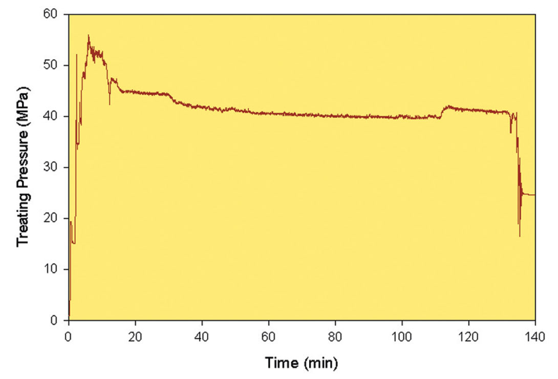
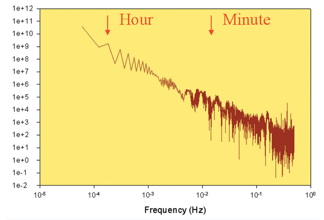
Hydraulic fracture stimulations utilize variable injection rates and associated pressures; however Figure 3 shows an example of what could be considered an average pressure record which is approximately uniform through the injection, and Figure 4 shows the corresponding frequency spectral content. Note that the pressure is what pushes the fractures open and so is directly linked with the fracture dilation. The plot shows that most of the power is at low frequencies corresponding to time periods of more than one hour. At increasing frequency, the associated power decreases. At seismic frequencies above 1 Hz (or time periods less than one second) there is a relative power decrease of over 8 orders of magnitude, relative to the lowest frequencies. Clearly the injection pressure is predominantly a slow process with most of the power that ultimately goes to fracture and eventually dilate the fractures occurring at frequencies much less than one Hz, in other words at much lower frequency than normal seismic monitoring.

Microseismic Deformation Frequencies

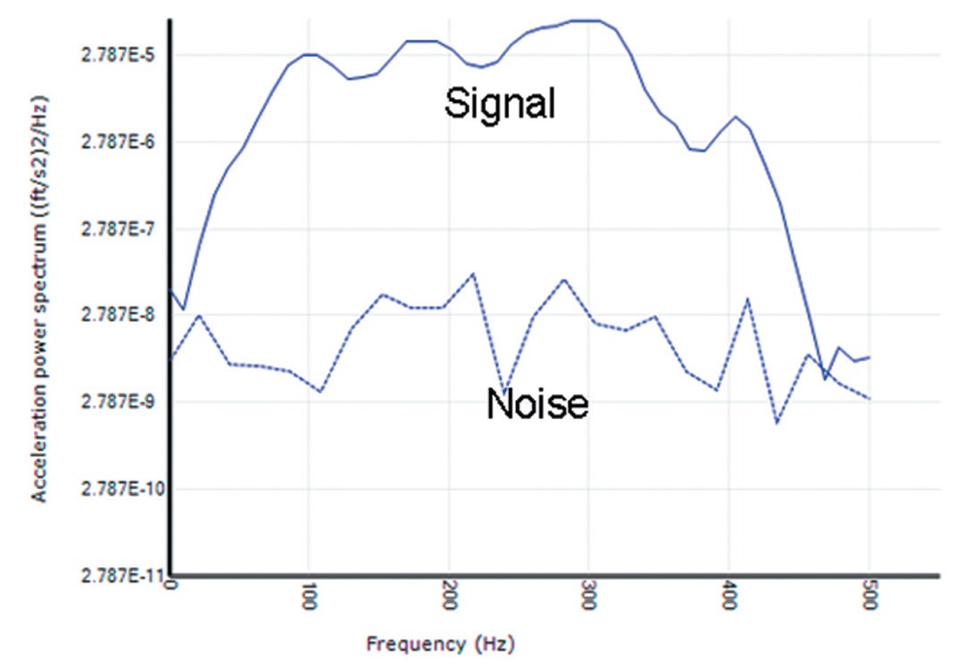
As indicated above, the normal frequency bandwidth of borehole microseismic monitoring is above 1 Hz, such that low injection frequencies are outside of the recording bandwidth. Low frequencies or time scales longer than 1 second can be recorded using broadband earthquake seismometers. Tiltmeters are also able to respond to very low frequencies and are occasionally used for hydraulic fracture monitoring, although respond to the overall fracture deformation compared to relative localized microseismic sources. Microseismic signal frequencies are typically relatively high frequencies in the range of 100’s of Hz (e.g. Figure 5 showing the relative amplitudes at different frequencies that constitute one of the microseismic signals of a located event shown in Figure 8). The microseismic source frequency is related to the slip time or area of seismic slip. The range of frequencies of recorded microseismic signals is also controlled by the frequency bandwidth over which the seismic sensors detect signals, generally in the 1 Hz to 1000 Hz range (or source deformations with time scales of a few milliseconds to a second) for most borehole microseismic recording arrays. Therefore, the normal microseismic recording is in a higher frequency band and outside of the average low frequency bandwidth of the pressure that drives the hydraulic fracture dilation.

Hydraulic Fracture Deformation Energy

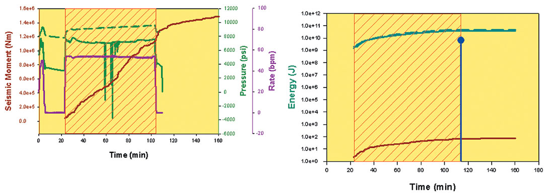
The energy or work associated with injection can be computed as the product of the injection pressure and volumes. Maxwell et al. (2008) describe several projects where the injection energy is calculated. Figure 6 shows the hydraulic energy computed for a specific case. In this example, the hydraulic energy was 50 gigajoules, or to give some physical context is approximately equivalent to the potential energy associated with dropping approximately 1000 railroad locomotives a height of 1 m. For this example, the microseismic locations suggested a simple, planar hydraulic fracture geometry which was calibrated with a fracture model (Maxwell et al., 2008). Based on the modeled fracture dimensions, the work done creating this fracture geometry is approximately equivalent to the total hydraulic energy of the injection, with the remainder of the injected energy being attributed to fluid leak off and frictional losses.

Microseismic Deformation Energy

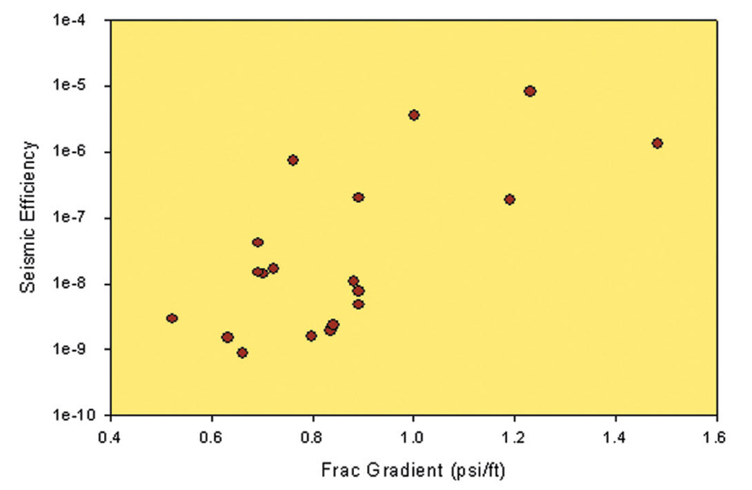
radiated seismic energy (total energy associated with microseismic events) can be computed by adding together the estimated seismic energy of individual microseismic events, or alternatively can be estimated from the cumulative seismic moment (Kanamori, 1978). Maxwell et al. (2008) describe a number of projects where the microseismic energy is compared with the hydraulic energy. In contrast to the hydraulic energy, the microseismic energy tends to be relatively small proportion. In the example described above, the total seismic energy was 100 J and roughly equivalent to the potential energy associated with dropping a mass of 10kg (22 lb) the height of 1m. Obviously in comparison with the pumped hydraulic energy is a relatively small portion of the total hydraulic energy. Maxwell et al. (2008) introduce a parameter termed the ‘seismic injection efficiency’ (SIE), defined as the ratio of microseismic to hydraulic energy. Note that this is different from seismic efficiency defined as the ratio of seismic energy to the local energy dissipation around the seismic source. For several projects, the SIE ranges between about one part in a million to one part in a billion (e.g. Figure 7), what can only be described as a very small part of the energy balance of the hydraulic fracture.

Rationalization of Hydraulic Fracture and Microseismic Deformation

To summarize the various aspects discussed above:

1. The hydraulic fracture is predominantly tensile opening; microseismic is often a shear dominated mechanism.
2. The hydraulic fracture is predominantly a relatively slow process (hours), where microseismic is a relatively fast process (milliseconds).
3. The hydraulic fracture is a predominantly high energy process, where microseismic is relatively low energy.

Therefore there are a number of paradoxes between the modes of the hydraulic fracture and microseismic deformations.

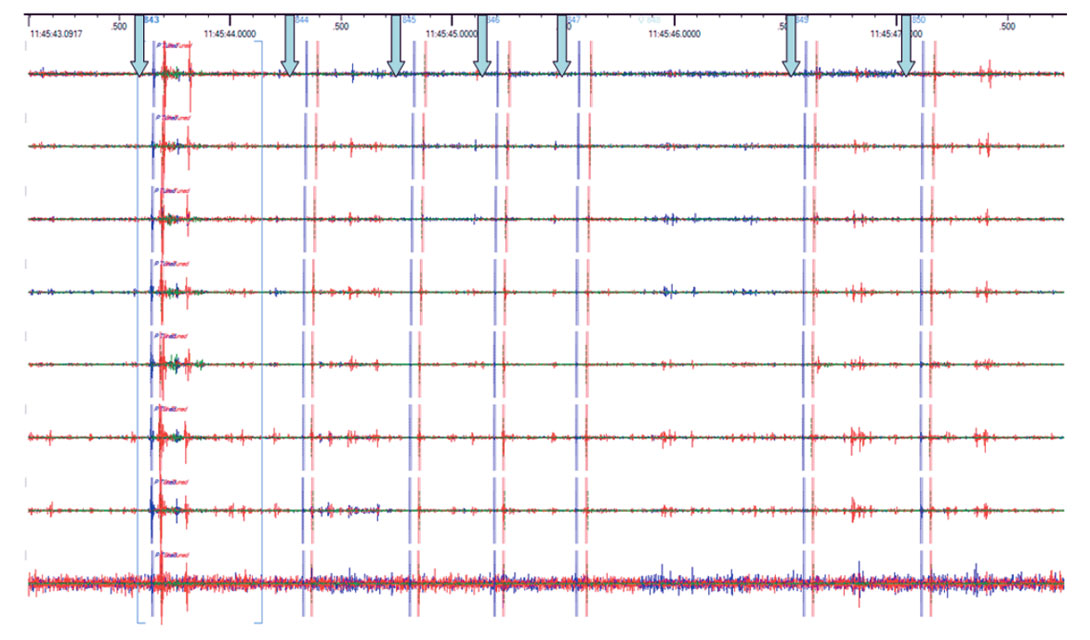
An important and relevant issue that has yet to be discussed so far is ‘aseismic’ deformation, which can be broadly defined as deformation without recording seismicity. One form of aseismic movement is microseismic signals similar in characteristic to the recorded seismicity but with amplitudes too small to be detected. Figure 8 shows a relatively long time window of seismic recording during a hydraulic fracture. Note the large number of signals similar in character to the detected and located microseisms, but much smaller amplitude. Within any microseismic monitoring project, there is a selection criterion that defines what microseismic signals can be confidently located: normally based on some constraint of minimal signal-to-noise ratio or identification of both p- and s-wave arrivals. Notionally these smaller signals are similar in source characteristics as the located microseismicity, and the lower amplitudes would account for diminishingly small contributions to the total radiated seismic energy. Slow opening modes would also be classified as aseismic, and could have different mechanisms and source characteristics to the microseismicity. Other authors (Warpinski et al., 2004) have argued for microseismicity being localized near to, but offset from, the hydraulic fracture where the paradox described above could be explained by the microseismic representing indirect deformation triggered by a slowly dilating hydraulic fracture and associated pore pressure changes. One likely form of this is induced stress activation (e.g. Maxwell et al., 2009) where stress changes associated with hydraulic fracture strains could activate or trigger deformation of a near-by fault or fracture. In the case of critically stressed faults, even a relatively slight stress change could induce fault slip. Regardless if the microseismicity is directly or indirectly associated with the hydraulic fracture there is clearly a significant amount of aseismic deformation in addition to the microseismic deformation.

An additional clue about the physics of the deformation associated with the observed microseismicity is related to its timing. In some cases, the microseismic deformation may not occur continuously during the frac, conversely increased seismicity levels could be recorded at the start, end, or at maximum proppant concentrations for example. Obviously increased microseismic activity rates say something about the underlying hydraulic fracture mode. However, in some cases there may also be a lack of seismicity during parts of the treatment during which time deformation must have occurred due to hydraulic fracture opening to accommodate the injected volume. Consider the hydraulic fracture example discussed in the energy balance section, as an example of the best case scenario where relatively continuous microseismic activity occurred through the injection. During the approximately 80 minute (or 4800 sec) frac, roughly 100 events were recorded. Assuming each microseismic event had a dominant signal comprising a pulse with average duration 5 ms (i.e. frequency of 200 Hz), then the total time intervals of microseismic source deformation represents about 0.5 sec. Relative to the total injection period, this deformation only represents 0.01% of the time, indicating a large temporal gap between these relatively instantaneous periods when microseismic deformation occurs. Further to this temporal gap there is also a significant spatial gap in the microseismic deformation relative to the hydraulic fracture. Based on frequency content, the radius of slip of the microseismic deformation can be estimated assuming a kinematic model of the rupture. The area of slip for the observed microseismic frequencies would be of the order of few m2 which represents a small surface area relative to the overall hydraulic fracture area (the frac is approximately 80 m high and 300m long or 24,000 m2). In this context the total microseismic slip area is about 100 m2 or 0.4% of the total fracture area. Hydraulic fracture deformation clearly must take place aseismically in addition to the spatially and temporally localized microseismic ‘snaps and pops’.

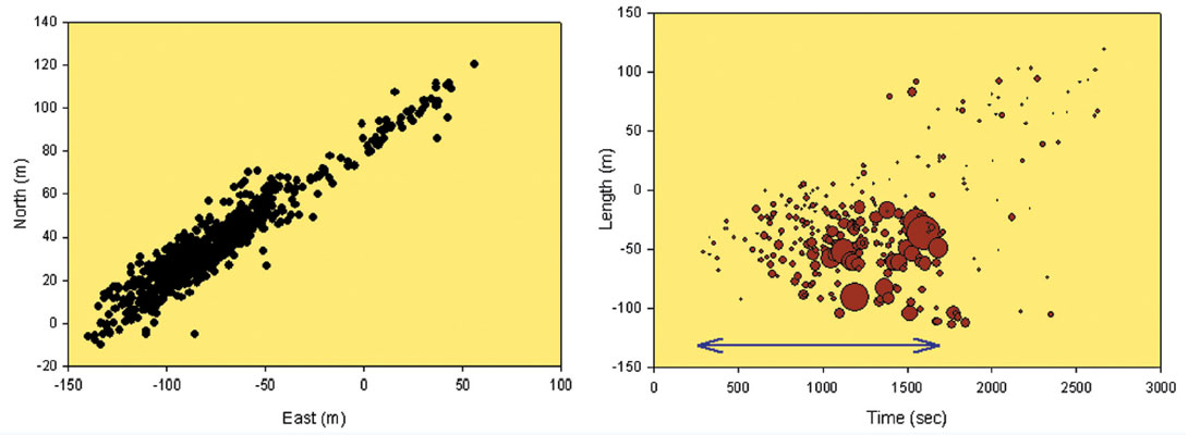
A final important piece of evidence about the nature of the microseismic deformation can be found by examining when the microseismic event occurs during the hydraulic fracture. Figure 9 shows a map view of a relatively planar microseismic image, along with the time of occurrence of the microseismic scaled by magnitude. The example demonstrates a few notable characteristics that can also be seen in a number of other microseismic monitoring projects. Firstly, relatively little activity occurs along the leading edges as the microseismic ‘cloud’ grows outwards. The majority of the microseismicity, including the largest magnitude events, occurs behind the leading edge. This same dataset is one of several included in Figure 2 and so is consistent with a strike-slip shear mechanism either parallel or orthogonal to the microseismic trend. It could be argued that the observed increased deformation is associated with pore pressure increases causing slip offset from the hydraulic fracture, although the dilation of a hydraulic fracture would tend to increase the compressional stresses and clamp fractures to resist shear deformation in these orientations. A more likely interpretation for this narrow band of microseismicity is that the microseismic deformation is directly related to the hydraulic fracture, and Figure 9 indicates that strength or intensity of the deformation increases with time.

Armed with these observations, we can now consider models that attempt to explain the microseismicity in context of the hydraulic fracture. Warpinski et al. (2004) discuss the shear deformation occurring at the tip of a hydraulic fracture. As indicated above, this is likely a mechanism of some microseismicity as regional stress changes result in induced shear deformation particularly from critically stressed fractures already close to the point of slipping. However, here we will limit the discussion to the region immediately around the hydraulic fracture. Based on the observed shear strike-slip mechanisms described above, two potential models are presented that are consistent with various observations previously highlighted. Both models assume that the microseismic is associated with the hydraulic fracture growing into, or possibly close to, a pre-existing natural fracture. While there are likely a wide variety of ways that a hydraulic fracture can form and grow, there are similarly a wide variety of potential microseismic mechanisms. Furthermore, a wide range of orientations of pre-existing fractures can exist, although here we will focus on end members either approximately parallel or orthogonal to the hydraulic fracture direction. However, the following discussion is meant simply to speculate about models that are consistent with the empirical observations noted previously. As such, at best the models can be viewed as possible dominant mechanisms for these specific examples.

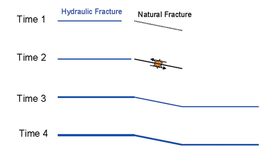
The first model involves interaction of the hydraulic fracture with pre-existing fractures subparallel to the hydraulic fracture direction (Figure 10). This model is similar to what is described by Rutledge et al. (2004) and Fisher and Guest (2011). As a hydraulic fracture (an implicit assumption here is that this is a tensile fracture that opens aseismically) grows into such a fracture, the normal stress can be decreased and the fracture could slip under shear. Assuming the hydraulic fracture is orthogonal to the minimum stress direction, the pre-existing fracture must be subparallel to it in order to have any resolved shear stress that can result in a shear slip. Note that the initial slip could occur before the hydraulic fracture grows into the natural fracture, but once the hydraulic fracture reaches the pre-existing fracture, slip will be a hybrid mechanism including tensile opening due to the pressurized fluid within the hydraulic fracture in addition to the shear. Recall that results shown in Figure 2 suggested largely shear deformation. Conceivably the microseismic slip could be associated with partial stress release, in which case additional microseismic events could be generated repeatedly at the same location. Once the hydraulic fracture grows through the pre-existing fracture, it would tend to dilate with the net injection pressure and potentially continue to deform in modes that contain some shear but the deformation would be slow and aseismic. The effective normal stress on the rock would decrease with time and hence the probability of instantaneous microseismic-type shear slip would diminish. This model may be a mechanism in some cases including a subset of the microseismicity described here, particularly at the leading edge of the microseismicity. However, this model appears to be unable to explain the increasing magnitude of events observed behind the leading edge of the microseismicity in Figure 9, suggesting other mechanisms. Furthermore, the model would not result in complex fracture networks like those observed in many shale reservoirs, although the model could explain the occurance of multiple subparallel hydraulic fractures if more than one hydraulic fracture grew out of a natural fracture.

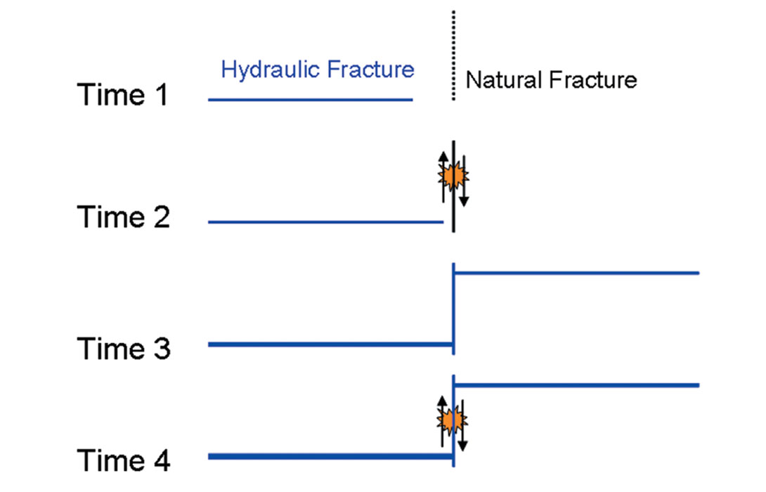
The second model is somewhat similar to the first, although the orientation of the pre-existing fracture is now orthogonal to the hydraulic fracture direction (Figure 11). This would represent a conjugate fracture set which has been attributed to the generation of complex fracture networks (see for example Gale et al., 2007). The models shown in Figure 10 and 11 could therefore both be relevant, since both fracture geometries could occur together. Geometrically this second model would be an example of a fissure type model (Cipolla et al., 2008). As before, the stress field around a hydraulic fracture could induce shear deformation prior to the hydraulic fracture reaching the pre-existing fracture. Again this would result in microseismic activity at the leading edge of a growing cloud of microseismicity, and is consistent with the inferred microseismic shear mechanism. As in the previous model, once the hydraulic fracture meets the pre-existing fracture the fracture will be pressurized. However, mechanically now there is one important difference resulting from the orthogonal geometry: dilation of this fracture will be restricted since it is opening against the maximum horizontal stress instead of the minimum horizontal stress. Furthermore, the fracture could build up additional stresses if the hydraulic fracture is offset through the pre-existing fracture (as described in Maxwell et al., 2009). The hydraulic fracture dilation on each side of the pre-existing fracture would increase shear strain and could result in stick-slip shear microseismic events. Indeed such events are consistent with so-called multiplets: repeating microseismicity with similar characteristic and locations (e.g. Raymer et al., 2008). This model could explain the microseismic occurring behind the leading edge of microseismic activity. Scenarios could also be conceived where the magnitudes would actually increase as shown in Figure 9, for example if the normal stress is maintained on the pre-existing fracture due to a Poisson ratio type effect from the compression associated with the hydraulic fracture dilation.

Compared to the previous model, this shear fissure model appears consistent with all the evidence presented here. The model also holds promise, in that it is directly analogous to transform faults along mid-oceanic spreading ridges (e.g., McGuire et al., 2005). Offsets in these often aseismic spreading ridges (where new oceanic crust is created during plate tectonics motion), result in strike-slip shear earthquakes along connecting spreading ridges. Similar to the fissure model, the majority of the deformation is aseismic, the energy balance is huge in moving the massive tectonic plate compared to the transform fault shear earthquakes, the seismic deformation is continually occurring and the earthquakes are on fault surface distinct from the main deforming spreading ridge.

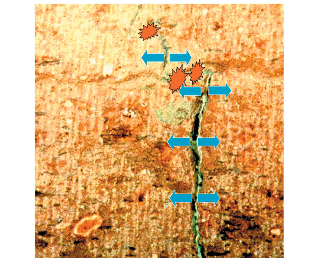
Finally, consider the hydraulic fracture photograph (Figure 12) from a mine-by experiment (Cipolla et al., 2008). The photograph has been annotated with the approximate location of hydraulic fractures and offset fissures (in this case likely bedding planes) which would be the site of induced shear deformation. Although microseismic was not recorded for this project, it seems likely that microseismic activity would occur along these fissures. Therefore, the speculative fissure model may be a relevant deformation model to reconcile microseismic and hydraulic fracture deformation. However, the orientation of the microseismic failures planes may not be the same as the conductive hydraulic fracture planes. If true this is obviously an important caveat when attempting to infer fracture orientation from microseismic mechanisms.

To summarize, consider again an ‘ideal’ seismic source such as a vibrator which has been specifically engineered to efficiently generate a seismic wave during reflection surveys. The vibrator is designed to mechanically vibrate in the desired seismic frequency band, is mechanically efficient with the majority of energy being concerted into seismic energy and is well coupled to the rock. In contrast, the over-riding objective of hydraulic fracturing is to stimulate production by creating a hydraulically conductive fracture to enable flow into the borehole. A hydraulic fracture is certainly not designed nor intended to be an efficient seismic source, and as described here does not meet the same source design criteria as a vibrator. Nevertheless the microseismic activity can be interpreted in terms of the hydraulic fracture geometry and be used as a measure of the stimulated volume as described in the next section. The deformation characteristics of the microseismicity are also important parameters and will ultimately enable calibration and validation of geomechanical models, once the context of the microseismic deformation is properly set in view of the overall hydraulic fracture deformation.

Stimulated Volume

A common microseismic measure is the created stimulated volume (here the contraction SV will be used, but is also termed SRV for ‘stimulated reservoir volume’ by Mayerhofer et al., 2008 or ESV for ‘estimated stimulated volume’ by Daniels et al., 2007). Typically, the spatial extent of the microseismic cloud is used to measure the SV: such that the SV is a measure of the volume of the microseismically active region. SV has become a fundamental metric of microseismic hydraulic fracture imaging projects. In this section, the components of the measured microseismic volume are briefly discussed and critiqued. Although the following discussion specifically addresses SV, the discussion can be generalized to determination of hydraulic fracture dimensions in specific directions: such as height and length.

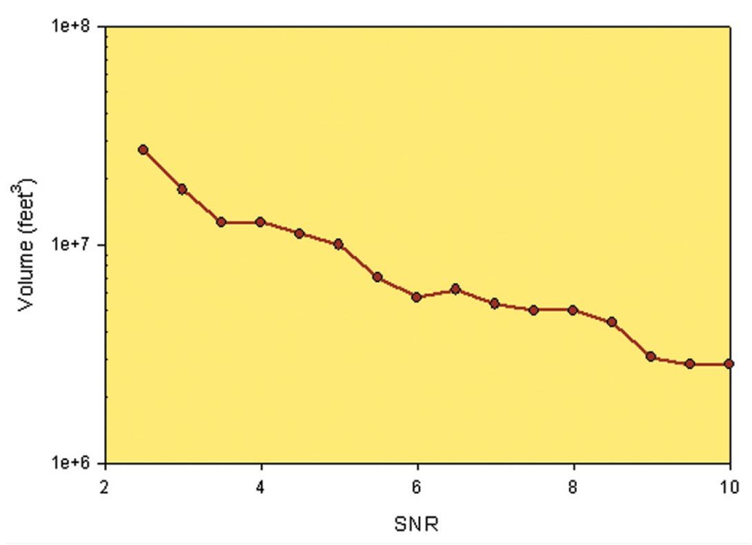
The microseismically active volume will reflect the total hydraulically created dimension, as the fracture growth causes geomechanical and associated microseismic deformations. The propped volume within this hydraulic fracture volume can potentially be estimated using a calibrated fracture model (e.g., Cipolla et al. 2010). However, the hydraulic fracture opening can also cause stress induced microseismic activity along structures not hydraulically connected (e.g., Maxwell et al. 2009), and hence the corresponding microseismic active volume could exceed the hydraulically created volume. In scenarios where critically stressed faults or fractures are close to the point of slipping, small stress changes associated with hydraulic fracture deformation can result in small changes in the local stress field and can result in remote activation of certain features. The volume of the microseismic cloud will also have associated measurement uncertainties and a tendency to overestimate the underlying deforming volume as shown in Figure 13, such that the larger the individual source location uncertainty the larger the microseismic cloud volume (Maxwell et al. 2010). This is potentially an important consideration in the confidence of the estimated SV: since the lower the confidence and more uncertainty in the microseismic locations, the larger the estimated SV. Therefore the microseismic location volume will be an overestimate of the microseismic deforming volume, and an upper limit on the extent of hydraulic.

Although the microseismic volume or SV can be larger than the hydraulic fracture volume due to uncertainty in the event locations and microseismic events generated due to deformation and porepressure effects, the microseismic events are likely proximal to the hydraulic fracture Although limited, the direct observation of hydraulic fracture geometry from core-throughs and field experiments indicate the microseismic images provide a good measurement of geometry for planar hydraulic fractures (Branagan et al,. 1996). Fracture length interpreted from microseismic images has also been consistent with observations of offset well pressure interference during production. When fracture growth is complex, direct observations of fracture growth are much more difficult, but there are documented cases where fracture complexity interpreted from microseismic images is confirmed by frac water “killing” offset wells. However, the detail of the underlying complex fracture structure is not easily interpreted from the microseismic image. Therefore, microseismic images alone can tell us a lot about the basic location and simple geometry (e.g. fracture length and height) of hydraulic fractures, but a more holistic approach is required to fully interpret microseismic images and extract hydraulic fracture structure.

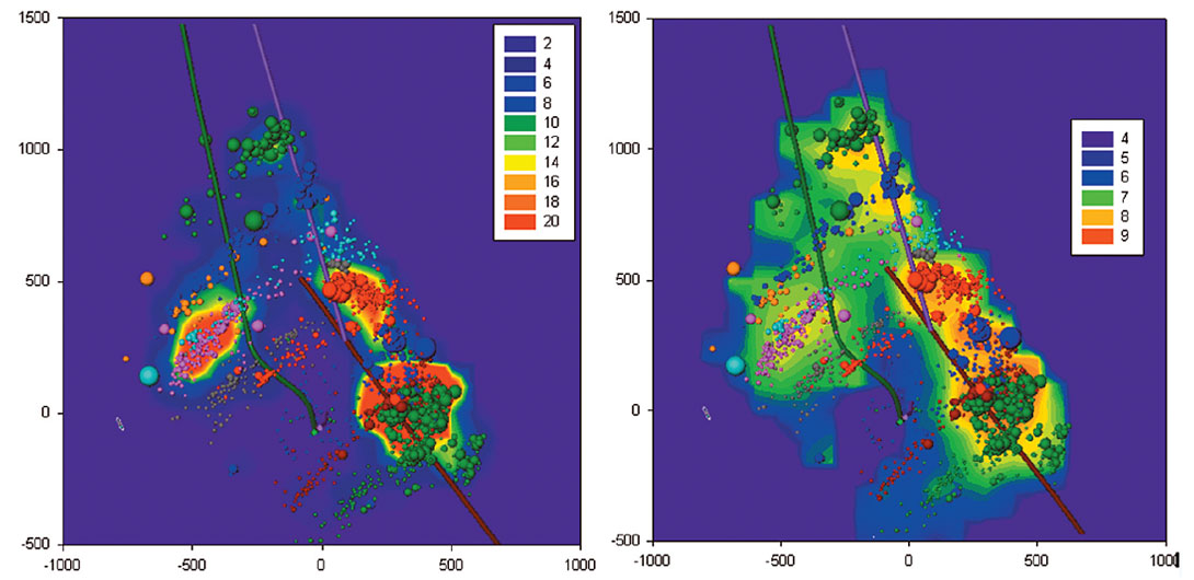
In addition to using the microseismicity to estimate the total SV, additional insight can also be gained about the variations in deformation within this volume. Consider how the volume of the microseismic cloud is typically estimated. Initial attempts relied on a simple, rectangular box (e.g., Mayerhofer et al. 2008) but evolved into more complex shapes to describe the extent of the microseismic cloud (Maxwell et al. 2006). Contours of event density can also be used, with the advantage that a threshold of event density can be used to deemphasize sparsely spaced and potentially mislocated events. Alternatively, seismic moment (source strength) density can be used to quantify the microseismic deformation density (e.g., Maxwell et al. 2003). Figure 14 shows a comparison of event density and deformation density. Deformation density is a more meaningful attribute than the event density and can help interpret fault activation and relative fracture density within the microseismic volume. For example, Figure 14 shows a fault activation example, where the high moment density along the NE edge is attributed in this case to fault activation (Maxwell et al., 2011). Seismic frequency analysis can be used to estimate the area of slip associated with each microseismic source, and with the seismic moment enable estimation of the seismic displacements that can be displayed in a similar contour plot. This deformation image can be directly interpreted in terms of variations in the density of pre-existing fractures or alternatively variations in the amount of localized hydraulic fracture dilation. In addition to the SV, such images provide additional information about variations in the density of microseismic deformation.

Microseismic Calibration of Geomechanical Fracture Models

The ability to simulate hydraulic fracture growth is a key element of frac engineering design. Hydraulic fracture stimulations can be modeled through a fracture mechanics model that simulates the fracture dilation/strain, leak-off, hydraulic conductivity and associated pressure profile for a given injection volume. Models are commonplace for relatively simple, planar, 2D fractures. In cases of complex fracture networks new methods are only now becoming available with capabilities to address creation of new hydraulic fractures and/or activation of preexisting natural fractures which result in coupled geomechanical and hydraulic interaction between individual components of the fracture network (e.g. Weng et al., 2011). Typical input parameters of a complex fracture model are the 1D or 3D stress state and mechanical properties of the rock and pre-existing natural fractures (a complete discussion of complex model is outside the scope of this paper, however Cipolla et al., 2010, provides more detail on key aspects related to microseismic). A description of the pre-existing natural fracture network is also required: in particular location, size and orientation. Various sources of information can be used to gain the input parameters, but the microseismic can also be used as a direct source of information about the active fractures. For example, microseismic locations can be used to define location and possibly orientation of pre-existing fractures, mechanism studies can also be used to define orientations and potentially microseismic slip areas can be used to define fracture sizes. Microseismic mechanisms can also be used to define stress orientations, and verify the direction of fracture movements. Therefore, in addition to calibrating or validating the geomechanical fracture model, microseismic can also be used as a source of input information. Obviously care is needed in the workflow to avoid potential bias through calibrating with microseismic data that is used to constrain both the input and validate the model output, in addition to caveats discussed earlier that microseismically active fracture may be different from the tensile hydraulic fracture. While microseismic calibration of a fracture model is not a new topic, in light of the paradox described earlier in the paper contrasting the microseismic and hydraulic fracture deformation, a discussion is warranted in terms of the impact of this paradox on the model calibration. As with previous calibration workflows, input parameters are adjusted until the modeled results match the microseismic data. The match could be subjective or quantified through calculation of an objective function.

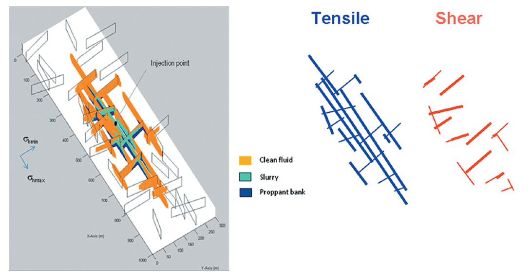
In order to compare the geomechanical simulation with microseismic data, a rock physics model is also required to define the microseismic deformation component of the total geomechanical deformation. The two mechanistic models described in the previous section represent such a rock physics model. The rock physics model defines the relationship between the total deformation and the component that matches the observed microseismicity, and thereby results in a synthetic estimate of the ‘modeled’ microseismic. The modeled microseismic deformation could conceivably predict the occurrence of individual microseisms or more likely a spatially continuous image of the estimated microseismic strain (similar to Figure 14). The rest of the discussion will focus on the later, and describe various workflows comparing such a simulated microseismic deformation strain field with comparable observed microseismic data. Figure 15 shows an example of a complex fracture model, along with potentially idealized microseismic deformations. Two realizations of potential microseismic deformation are shown: one assuming that the ‘microseismic’ responds to tensile opening from either creation of new hydraulic fractures or dilation of pre-existing fractures, and the other assuming ‘microseismic’ corresponds to shearing as described previously in relation to both Figures 9 and 10. For illustration purposes, the relative amounts of deformation are also approximated (shown by the line width), by assuming more tensile deformation in the minimum stress direction and more shear deformation along pre-existing fractures between hydraulic fractures. Contrasting these two realizations (Figure 15) points to the need to properly understand the rock physics model in order to define what component of the deformation is captured with the microseismic, as well as what is not captured.

Basic calibration of the fracture model is often limited to matching the 3D extent or ‘footprint’ of the stimulated volume based on microseismic locations. Such a calibration (Figure 16) could involve either matching the entire microseismically active region during the job (i.e. matching the final end-of-job footprint) or the temporal behavior by matching the dynamic growth through evolution of the footprint during the stimulation. Temporal growth could be matched by comparing the SV with time. Additional information can improve the match by comparing the spatial/temporal variation within the SV, for example using the event density or more appropriately microseismic deformation densities (see for example Figure 14). Contours of the microseismic displacements are believed to be the most robust parameter form comparison, since it can be compared directly to simulated strains in the geomechanical model. More sophisticated calibration could potentially extend the scalar displacement comparison to match the tensor strain deformation through microseismic mechanisms of the direction and possibly mode of displacement.

The comparison could either be qualitative by attempting to match the relative extent and variability of the deformation in terms of localized clusters, or possibly be truly quantitative by matching the absolute displacements. A complete deterministic and quantitative match is a significant challenge, and would require calibration of seismic efficiency and the amount of aseismic deformation. Furthermore, the microseismic events can represent a partial stress drop or slip on just part of the stressed fracture surface further complicating a quantitative match. However, the energy balance between the injected hydraulic energy, modeled deformation energy and modeled and observed ‘microseismic’ energy could be used for quantitative calibration. The potential advantage of comparing the energy balance is that it provides a method to calibrate the overall seismic efficiency and details about how the strain is released through the microseismicity. Studies of tectonic faults face a similar challenge in understanding the quantitative seismic strain, and often use geodetic information about the total strain field represented by the local tectonics motions to provide context to earthquake data. The analogy here is to use the hydraulic energy as a proxy to the total strain.

Once calibrated, the fracture model can be used in reservoir simulation for a production history match (e.g. Cipolla et al., 2010). In this way, the hydraulic fracture effectiveness can be examined and potentially be improved to enhance well or reservoir performance. Since the microseismic deformation is just one component of the total deformation, this geomechanical model calibration is a critical step in the workflow and avoids potential pitfalls in trying to assess the fracture effectiveness directly from just the microseismic deformation.

Conclusion

The microseismic source strain deformation provides an image of one aspect of the hydraulic fracture deformation. Examples presented here point to a paradox between the microseismic and hydraulic fracture, where the microseismic is a relatively fast, shear fracture mode while the hydraulic fracture is a relatively slow, tensile opening mode. The differences in these modes of deformation can be resolved by realizing the significance of aseismic deformation. Comparisons of the energy balance between the microseismic and injection shows that the majority of the hydraulic fracture deformation is aseismic and not captured by the microseismic. The paradox in deformation modes implies that aseismic deformation is closely associated with the hydraulic deformation which ultimately will be the main control on the fracturing process and effectiveness. Therefore the microseismic deformation does not provide direct information about the hydraulic fracture effectiveness, although can be used to constrain a geomechanical model by defining the rock physics that controls the context of the microseismic strain.

The geomechanical model calibration can use various levels of sophistication: from a basic match of the footprint of the extent of microseismicity, temporal evolution of the footprint, spatial variations in the scalar microseismic slip displacements, and ultimately to include a match of the directional slip displacements. These calibration workflows can either be in a relative sense in an attempt to qualitatively match the spatial and temporal strains, or a completely quantitative match. The full quantitative match between observed and modeled microseismic strains requires additional attributes such as the energy balance between the microseismic and injection energies, to calibrate the seismic efficiency and aseismic components. Nevertheless, a calibrated geomechanical fracture model can then be used to examine the hydraulic fracture effectiveness and enable confident incorporation into a reservoir simulation model.