Reverse-time depth migration in elastic media

The main objective of this paper is to sketch a reverse-time migration workflow. The migration is based on an elastic model of the earth, is driven by elastodynamic equations, and processes mutlicomponent seismic records. It works with shot gathers and is a prestack migration. As a typical depth migration, the kernel of its algorithm transforms input surface records in time to wavefield snapshots in depth before imaging conditions are applied, and the outputs are images in depth. This work is based on the author’s 2012 Ph.D. dissertation.

Introduction

Seismic imaging technologies have progressed to the point where depth imaging of elastic waves, recorded using multicomponent data, can be achieved – although time or depth acoustic imaging of single component data is still the workhorse for most processing. The motivation for using multicomponent surveys and elastic imaging is that the earth is more accurately approximated by elastic media than it is by the acoustic media assumed during single component imaging. The promise of elastic imaging is a more complete characterization of the subsurface and better estimation of reservoir properties.

The leading method of imaging today is Reverse-time Migration. Despite the name, Reverse-time Migration, or RTM, is in fact a depth migration. The “time” in the name refers to the propagation method, whereas the domain of output is depth, as for other depth migration methods. More fundamentally, RTM honours wave propagation fully. Gray et al. (2001) stated: “We take the view that, roughly speaking, ‘time migration’ refers to migration algorithms that pay no attention to ray bending, and ‘depth migration’ refers to algorithms that do honor ray bending.” The authors were primarily considering different ray-based methods: namely straight ray approximations vs depth-model based ray paths which honour ray-bending. Though RTM doesn’t explicitly use concepts of rays and ray-bending, it does, like earlier finite difference methods of migration, implicitly take account of the full wavefield propagation effects, including all ray-bending effects due to changes in the elastic media. In contrast to standard acoustic RTM, which uses the scalar wave equation, elastic RTM is driven by the elastodynamic equations.

This paper addresses three aspects of RTM which are discussed in greater detail in the author’s Ph.D. dissertation (Jiang, 2012): wavefield modelling; computational boundaries; and a workflow for reverse-time migration. The source scheme and free surface boundary conditions are also briefly noted.

Forward modelling of the wavefield is a critical part of any RTM algorithm, as the downgoing wavefield must be modelled from the source position. Additionally, the reverse-time extrapolation of the recorded data, which gives the algorithm its name, also uses the same modelling formula, but simply run backwards. Here, a finite-difference algorithm using a staggered-grid (Virieux, 1986) is adopted, and its relationship to other related wave equation schemes is briefly described.

The computational boundary problem has been a persistent topic in the literature of wavefield modelling, and it is unavoidable in reverse-time migration as well. Computational boundaries are subsurface model boundaries. They differ from the physical boundaries in the model. For example, for a 2D subsurface model in the shape of a rectangle, the physical boundaries are a free surface on the top and rock boundaries inside the subsurface, while the computational boundaries are a bottom boundary and two sides on the left and right. The “problem” is that these boundaries can generate unwanted reflections which contaminate the modelled data. After examining two of the most popular solutions to the problem, absorbing boundary conditions and a nonreflecting boundary condition, a method combining these two solutions is proposed. The proposed hybrid method results in fewer boundary reflections without extra computational costs.

The nature of the algorithm naturally means that RTM leads to different workflows than those for Kirchhoff migration. RTM has three components: wavefield forward modelling; wavefield reverse-time extrapolation; and application of imaging conditions. As noted earlier, the reverse-time extrapolation uses the same algorithm as forward modelling but with time reversed. In the author’s thesis, new imaging conditions were proposed, referred to as “source energy normalization imaging conditions”. There are other unique aspects to the RTM workflow: for example, ground roll suppression is not a necessary part of it.

Often in multicomponent processing the vertical component is taken as equivalent to PP and the horizontal component as equivalent to PS. These are approximations based on the assumption of near vertical arrival at the surface. In reality the P-wave arrival is measured on both vertical and horizontal components. To maintain clarity, these approximations are not adopted in this paper – instead the vertical and horizontal nomenclature is reserved for the actual components, whereas PP strictly refers to a reflected P wave from an incident P wave, and likewise PS refers to a reflected S wave from an incident P wave.

Wave modelling in elastic media

Equations describing waves in isotropic elastic media include three categories of relations: displacement-stress relations (Newton’s second law of motion), stress-strain relations (Hooke’s law), and displacement-strain relations. They are given as following:

where u is displacement, σ is stress, e is strain, λ and µ are Lamé coefficients, ρ is density, and D = Σ_ke_kk is the dilatation.

The above system of equations describes a three component wavefield in a 3D volume. Special cases of the above equations describe different wave modelling cases: from 1D to 3D, from non-staggered grids to staggered grids, from displacement only scheme to velocity- stress scheme. For example, two classic wavefield modelling cases studied by Virieux (1984, 1986) are obtained using 2D versions of this system with staggered-grid schemes: (1) considering a wave travelling in the plane of x₁ - x₃, with the particle vibrations perpendicular to the plane, one gets the 2D SH-wave case (Virieux, 1984); (2) considering a wave travelling in the plane of x₁ - x₃ with the particle vibration inside the plane, one gets the 2D P-SV case (Virieux, 1986). In both cases particle velocities are time derivatives of displacements, and stresses are the wave modelling output. Among different cases that have been studied, the 2D P-SV modelling method is selected and used for the reverse-time migration in this paper.

Having discussed the wave propagation scheme, the source scheme and free surface boundary methods should be briefly mentioned, each adapted for the elastic case. The methods used for the source and surface boundary conditions are those described in Manning (2008), and a Ricker wavelet is used for the source wavelet.

The more challenging problem of computational boundaries has been a continual subject of research in wave equation modelling, and requires more detailed attention. In the next section, two widely used approaches to this problem are analysed before a new hybrid approach is proposed and demonstrated.

Computational boundary conditions

The finite difference modelling method used in RTM takes place on a grid with regularly spaced nodes. At each step in the modelling the wavefield at each node is updated, using values at surrounding nodes. However, some of the surrounding nodes are not available for nodes on the model edges. The computational boundary problem arises on these edge nodes of the subsurface model.

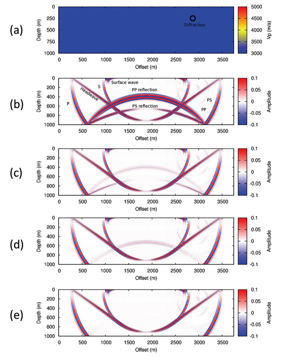
An intuitive solution is to set the boundary node wave values to zero since it could not be calculated. However, by doing that the boundaries act like physical rigid boundaries. A rigid boundary is an idealized immovable interface, with an infinitely large impedance. A little mental math tells us that the reflection coefficient upon this boundary is 1. Thus, one can predict that waves striking such a boundary produce no motion of the boundary particles at all, and all the seismic energy is reflected back. This can be confirmed by numerical modelling as well. Figure 1a shows an isotropic medium containing a single point diffractor. With a seismic source at the surface centre, waves are generated and propagate down into the subsurface (Figure 1b). Wave diffraction happens at the point diffractor, and wave reflection happens upon the rigid bottom. The reflections upon the point diffractor are much weaker than the bottom reflections. To better study the physical waves masked by the artificial boundary reflections, it is necessary to suppress the latter. The computational boundary conditions problem, if not well dealt with, could severely damage the modelling results.

Fortunately, there are many solutions to the boundary condition problems. The most cited one is the “absorbing boundary conditions” proposed by Engquist and Majda (1977), and Clayton and Engquist (1977). Another popular method, called the “nonreflecting boundary condition”, was presented by Cerjan et al. in 1985.

The absorbing boundary is based on the separation of waves in different directions. This is accomplished by wave equation approximation. For the bottom boundary of a subsurface model, one can separate the upgoing and downgoing waves for vertically propagating waves. Once the upgoing and downgoing waves are separated, one may approximate the bottom node wavefields with only downgoing waves, so that at a later time the inside node modelling will not be affected by the upgoing waves. By doing so, it seems that the artificial reflections from the model bottom are absorbed by the boundary.

A nonreflecting boundary condition employs a strip of nodes on the boundary to attenuate wave amplitudes. These strips are also termed as “numerical sponges”. This method is straight forward, but it is more computationally expensive than the absorbing method.

Both the absorbing and nonreflecting boundaries cannot completely remove all the artificial reflections, however. The absorbing boundary works well only for waves moving perpendicular to it, since the separation of waves in the opposite directions can be relatively accurately done in this case. For waves that strike the boundary with other angles, the separation is less accurate, and more energy is still wrongly reflected (Figure 1c). For the nonreflecting boundary the attenuation of the wave amplitudes implies a property change of the medium to the wave equations which drive the modelling system, and also results in artificial reflections (Figure 1d). It is possible to choose different parameters, such as a thicker numerical sponge zone and a less aggressive attenuation rate, to minimize the artifacts, but that will be at the cost of much greater computational effort.

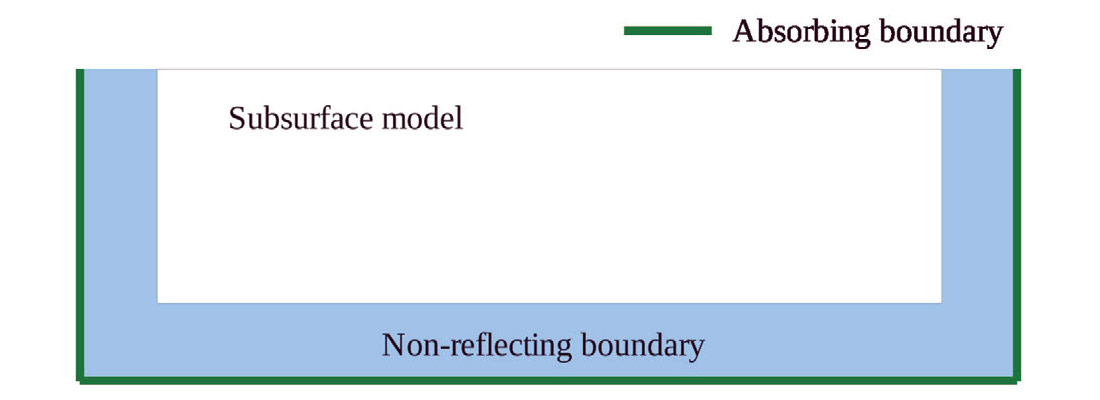
By combining absorbing boundary conditions at the outside boundary of the nonreflecting sponge strip (Figure 2), boundary reflections can be further reduced (Figure 1e) without any extra computational costs compared to the nonreflecting method.

Reverse-time migration

There are four main steps in the prestack reverse-time migration workflow (Figure 3). The workflow is quite different to Kirchhoff migration related processes.

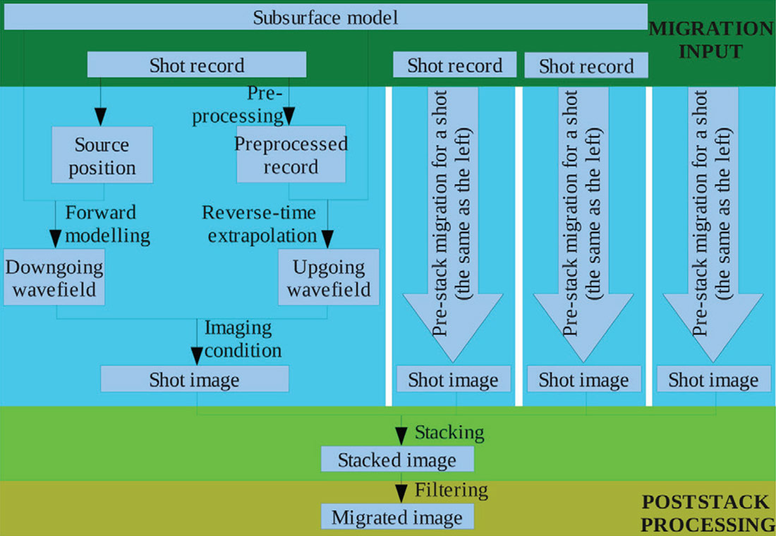
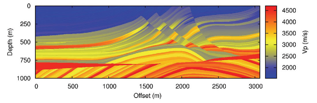
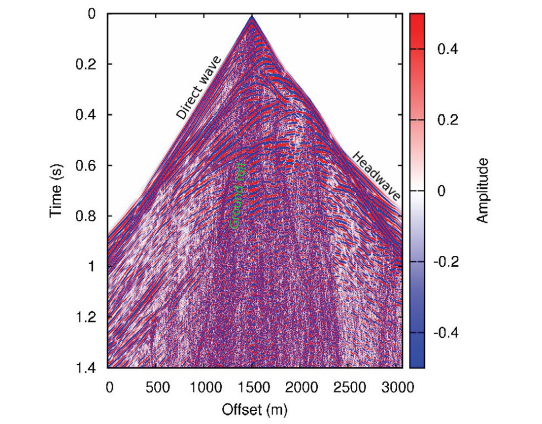
The first step is to acquire surface records and to build a subsurface model. In a real seismic survey, surface records are acquired from field seismic experiment. Then a subsurface model can be built from well logs, velocity analysis from surface record, full waveform inversion, and so on. In my numerical experiment, the subsurface model is a shrunk Marmousi2 model (Figure 4), and the surface records of particle displacement velocities (Figure 5) are “acquired” from numerical modelling using the subsurface model. Typical waves, such as direct arrivals, headwaves, ground roll, and reflections are observable on the record.

The second step is reverse-time migration of shot records, which includes forward modelling, reverse-time extrapolation of surface records, and applying imaging conditions.

Wavefield forward modelling provides the source wavefield for imaging. The physical properties of the subsurface media directly used in the modelling system are Lamé coefficients and density (the Lamé coefficients are derived from P- and S-wave velocities and densities). The output of modelling is a series of “snapshots” of the source wavefield as a function of the two spatial coordinates which describe the subsurface, for different propagation times.

In the literature, the source wavefield is sometimes called downgoing wavefield (such as by Claerbout, 1971).

With shot records as the input, snapshots of the receiver wavefield (sometimes called the upgoing wavefield) are obtained by reverse-time extrapolation. The surface records in time are transformed to wavefields in depth by this process. The extrapolation formula are the same as the modelling system, but the time sequences are reversed.

The only preprocessing of the shot records before reverse-time extrapolation is muting direct waves and headwaves that are mixed with direct arrivals. Removal of surface waves is not critical for reverse-time migration by nature: energy will imaged onto the final migration section only when the downgoing and upgoing wave energy meet at the same time and the same spatial position during both forward modelling and reverse-time extrapolation, but surface waves never go deep into the earth, as the name suggests, so it will only affect the migration result for the very shallow part.

Imaging conditions are used to correlate the source and receiver wavefield snapshots to get the subsurface images. Similar to the acoustic case by Whitmore and Lines (1986), imaging conditions can be developed for the 2D P-SV case. However, for the elastic case there are five imaging conditions instead of one:

where S and R, respectively, denote the source and receiver wavefields, V and H, respectively, denote the vertical and horizontal components, and I denotes the image at a certain subsurface position. The denominators on the right are the sum of zero-lag auto-correlation of both source components, which help eliminate source signatures. Figure 6 shows a centre shot image resulted from the VV imaging conditions.

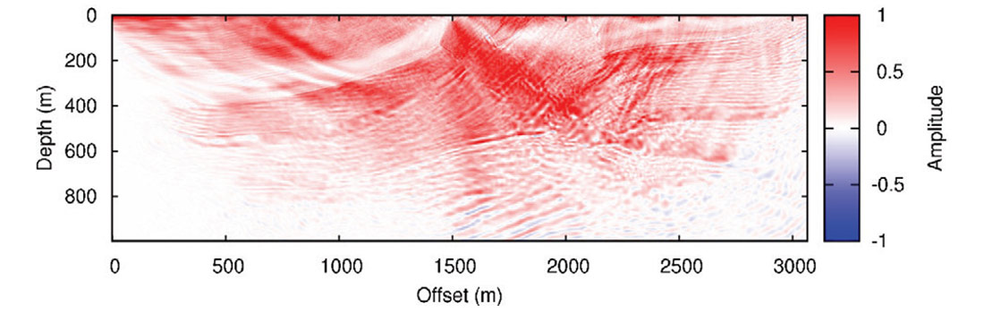
The third step is stacking shot images obtained from the second step. An image resulted from a single shot, such as the one shown Figure 6, shows obvious signature of the acquisition geometry: the central part beneath the source location shows stronger amplitudes. With shot image stacking, the acquisition signature and other types of non-coherent noise are attenuated: Figure 7 is a stacked image obtained from 49 shot images resulted from the VV imaging conditions. The stacking process greatly improves the signal-to-noise ratio.

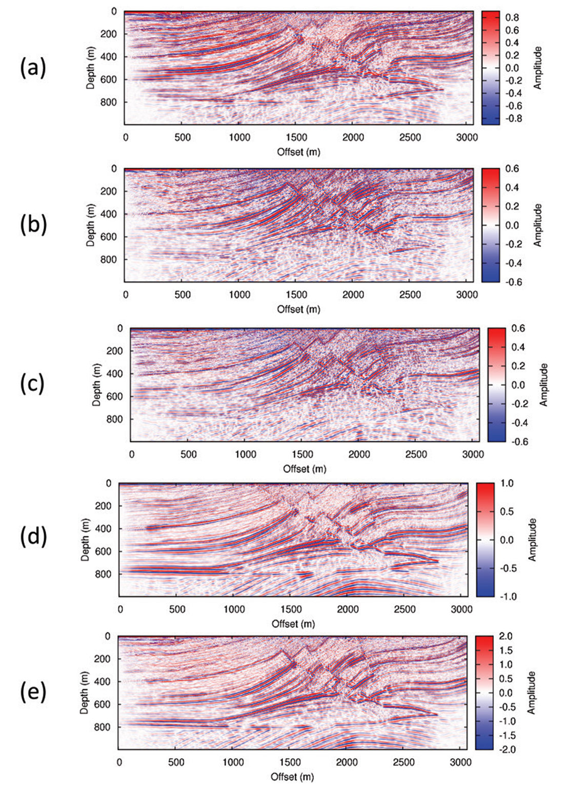
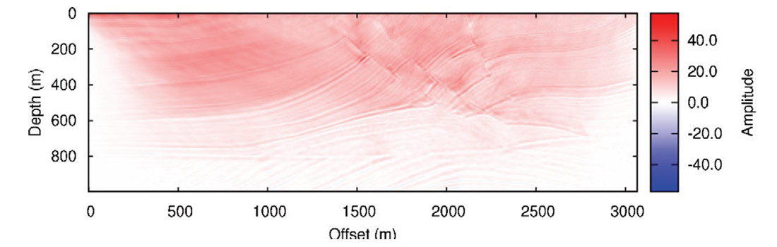
The fourth step in the workflow is to apply a high-pass filter to the stacked image to remove the very low frequencies (close to the DC component) in the stacked image. The image in Figure 8d is obtained by filtering the section shown in Figure 7.

The migrated sections (Figure 8) show different features in terms of depths of penetration and resolutions. Among the first four images, The VV image (Figure 8d) shows the deepest depth of penetration. This is reasonable: usually P waves are the main contributors to the vertical component in seismic surveys, and with faster velocities they reach deeper structure within a given recording time. As far as seismic resolution, the HH and VV images (Figure 8a, d) provide better vertical resolutions, while the HV and VH images (Figure 8b, c) provide better horizontal resolutions. Overall, the stacked section (Figure 8e) best represents the subsurface model (Figure 4), and shows a balanced resolution in both vertical and horizontal directions.

Summary

A workflow of a reverse-time depth migration in elastic media is sketched. The kernel of the workflow is the wavefield modelling algorithm, which is used to get both downgoing and upgoing wavefields in depth for imaging. As for the persistent problem of computational boundaries in wavefield modelling, a method combining absorbing and nonreflecting boundary conditions can effectively attenuate artificial boundary reflections without extra computational costs. Five imaging conditions developed for the elastic context result in different resolutions in the horizontal and vertical directions, and this can be helpful in interpreting structures with different dip angles.

Acknowledgements

The author would like to acknowledge to his Ph.D. supervisors, John C. Bancroft and Laurence R. Lines, and the other CREWES members for guidance and supports.

Thanks also go to several Key Seismic colleagues. Special thanks to Bernie Law and Richard Bale for their help and support.