Least squares migration of converted wave seismic data

Least squares migration permits the estimation of subsurface models that honor the recorded primary seismic wavefield. In addition, it permits us to include regularization constraints that reduce sampling and illumination artifacts. Least squares migration utilizing one-way wave equation migration has been mainly restricted to imaging via scalar wave propagation operators. We present an extension of wave equation least squares migration for vector wave fields. Synthetic results demonstrate that converted wave least squares migration can improve the resolution of PP and PS images, and can also be used for interpolation and wavefield separation.

Introduction

Converted waves are a useful tool for characterizing the elastic properties of a reservoir for a number of reasons. The comparison of PP and PS reflectivities can help us identify fluid contacts, and S-wave ray paths provide a tool to illuminate targets hidden beneath gas filled zones. Perhaps most importantly, P and S waves provide complementary information that is helpful when inverting for elastic parameters (Stewart, 1990).

Prestack migration is a critical step in the processing of converted waves. For P-wave seismology it is common to approximate wave propagation using the scalar wave equation. This approximation is often sufficient to produce reasonable P-wave structural images. Extending this approximation to converted wave imaging requires some troubling assumptions about amplitude and polarization. Migration algorithms based on the elastic wave equation more accurately model wave propagation and allow multiple wavefields to be imaged simultaneously. There are a variety of approaches to elastic migration. Kuo and Dai (1984) developed an elastic implementation of Kirchhoff migration. Chang and McMechan (1987) applied Reverse Time Migration (RTM) to multicomponent data using an elastic finite difference algorithm, resulting in horizontal and vertical component images. Dellinger and Etgen (1990) proposed the application of Helmholtz decomposition to elastic data using a Fourier domain operator. Later implementations of elastic RTM use this idea to provide distinct PP and PS images (see for example Yan and Sava, 2008). Extensive work has also been done on wave equation based methods to migrate elastic data. Xie and Wu (2005) used an elastic version of split step migration to downward continue elastic data, while Bale (2006) modified the phase shift migration to handle anisotropic elastic wavefields. Wave equation based methods are an attractive option because they perform more accurately than ray-based methods, and are much less computationally expensive than methods that employ finite differences. For example, in time domain RTM many wavefield snapshots for all time samples must be generated and saved prior to imaging, whilst in wave equation migration individual frequency slices are treated independently and the wavefield is recursively updated with depth.

The migration of converted waves comes with some additional complications when compared with P-wave migration. Typically PS data have a lower signal to noise ratio than PP data, and a slower S-leg gives converted waves an asymmetric ray path. While this implies that converted wave data have more restrictive aliasing criteria, it also presents an opportunity: given the same acquisition geometry converted waves can image the subsurface with a wider source side aperture than P-wave data. Furthermore, ignoring the effects of attenuation, a given frequency of converted wave data images the earth with a higher resolution than P-wave data. Realistically, attenuation is always a factor (especially in the near surface), which challenges the resolution of both PP and PS depth images (Bale and Stewart, 2002). Some of these challenges can be dealt with before migration. For example, regularization can be applied to reduce the effects of acquisition footprint on the migrated image (Cary, 2011). In this article we aim to address some of the challenges facing converted wave migration via least squares inversion.

Least squares migration, in its various forms, has been an active field of research for many years. Lambaré et al. (1992) used an iterative data fitting approach to solve for reflectivity. Nemeth et al. (1999) applied least squares migration with a Kirchhoff operator to image in the presence of poor spatial sampling, while Kuehl and Sacchi (2003) used regularized least squares wave equation migration to generate angle gathers that are unaffected by acquisition footprint. Wang (2005) and Wang et al. (2005) explore the application of 3D wave equation least squares migration with constraints to a real data set of the Western Canadian Sedimentary Basin. In a subsequent contribution, Wang and Sacchi (2007) also explore the incorporation of a sparsity constraint to least square migration to the ubiquitous problem of vertical resolution enhancement. Least squares migration of structurally complex data has been also being investigated via the utilization of preconditioning operators that were synthetized with prediction error filters (Wang and Sacchi, 2009). A common theme of all least squares migration algorithms is data fitting which depends greatly on the ability of the migration operator to accurately propagate energy from source to receiver. Extending least squares migration from the acoustic to the elastic case is a natural progression in data fitting.

Recently, Stanton (2014) proposed using Least squares prestack time migration to image and regularize converted waves. In this article, we tackle the more complex problem of utilizing Least squares migration with wave equation prestack depth imaging operators. We implement least squares migration using an elastic shot profile wave equation migration operator with an angle gather imaging condition. We use a synthetic data example to demonstrate that the algorithm can improve the resolution of PP and PS images. The algorithm can also be used for interpolation and wavefield separation.

Methodology

Least squares migration aims to find a migrated image that minimizes the difference between observed and predicted data. The cost function for least squares migration of acoustic data with quadratic regularization is

where T is a sampling operator, L is a forward (demigration) operator, m is the migrated image we wish to solve for, and d are the observed data. We minimize equation 1 using Conjugate Gradients. Each iteration of CG involves applying the forward operator to predict data from the migrated image, computing a data residual, and migrating the residual using the adjoint operator to compute an update to the image.

Before adapting equation 1 to the elastic case we must first define our elastic migration operator. We form an elastic migration operator by combining Helmholtz decomposition with a wave equation migration operator that extrapolates P and S scalar potentials independently.

Isotropic elastic data can be decomposed into P and S-wave potentials by taking the divergence and curl of the wavefield components respectively:

This is commonly referred to as Helmholtz decomposition. Etgen (1988) evaluated these derivatives by Fourier transform. Writing this as a linear operator:

where F_x and F_x^–1 are the forward and inverse Fourier transform on the spatial axis respectively. In this equation the lateral wavenumber is given by k_x, and the vertical wavenumbers k_z(v_p) and k_z(v_s) depend on the P and S wave velocities of the near surface. Technically this upper layer should have a constant velocity, but practically we find that the average velocity is generally a good approximation.

After wavefield separation we extrapolate P and S wave scalar potentials using a shot profile wave equation migration operator with an angle gather imaging condition. To generate images m_pp and m_ps simultaneously, we can write

where L^T_pp and L^T_ps implement split step wave equation migration (Stoffa et al., 1990) of PP and PS images respectively. Split step migration consists of downward continuing the wavefield by depth increments using a phase shift determined using a background velocity, and performing a correction for the perturbation of the background velocity at each lateral position. The source is extrapolated using the P wave velocity. On the receiver side, operator L^T_pp extrapolates using the P wave velocity, while operator L^T_ps extrapolates using the S-wave velocity. Typically in wave equation migration the source and receiver are moved to a coincident position in the subsurface (migration to zero offset). To do this we extrapolate source and receiver wavefields and cross correlate them once for each lateral position we wish to image. After migration, all shots are summed to form the image. Forming angle gathers requires a small adjustment to this procedure. Instead of simply cross correlating the extrapolated source and receiver wavefields once at each lateral position, the cross correlation is repeated several times for different spatial lags. These lags can be interpreted as the subsurface offset between the two wavefields. Individual shots are stacked after migration and the offset axis is converted to angle using the relation

where γ is the half opening angle, and tan and tan are are the wavenumbers for the offset and the depth axes respectively (Rickett and Sava, 2002). For a more detailed derivation of the forward and adjoint operators in least squares shot profile migration, we refer the interested reader to Kaplan et al. (2010).

Using the wavefield separation and migration operators defined above, we can combine them to form the forward and adjoint operators needed for inversion. To forward model two component data we use

Conversely, to migrate two component data we take the adjoint of the forward operator to get

Finally, for elastic least squares migration with quadratic regularization the cost function is written

Again, this cost function can be minimized using CG. To improve convergence we can add preconditioning to suppress crosstalk artifacts in the angle domain using an FK fan filter.

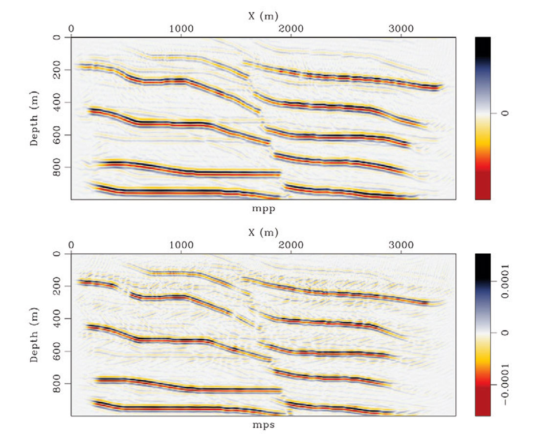
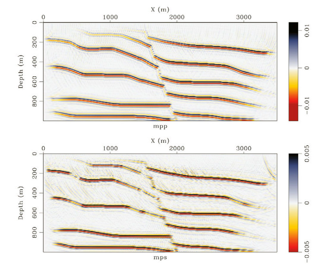
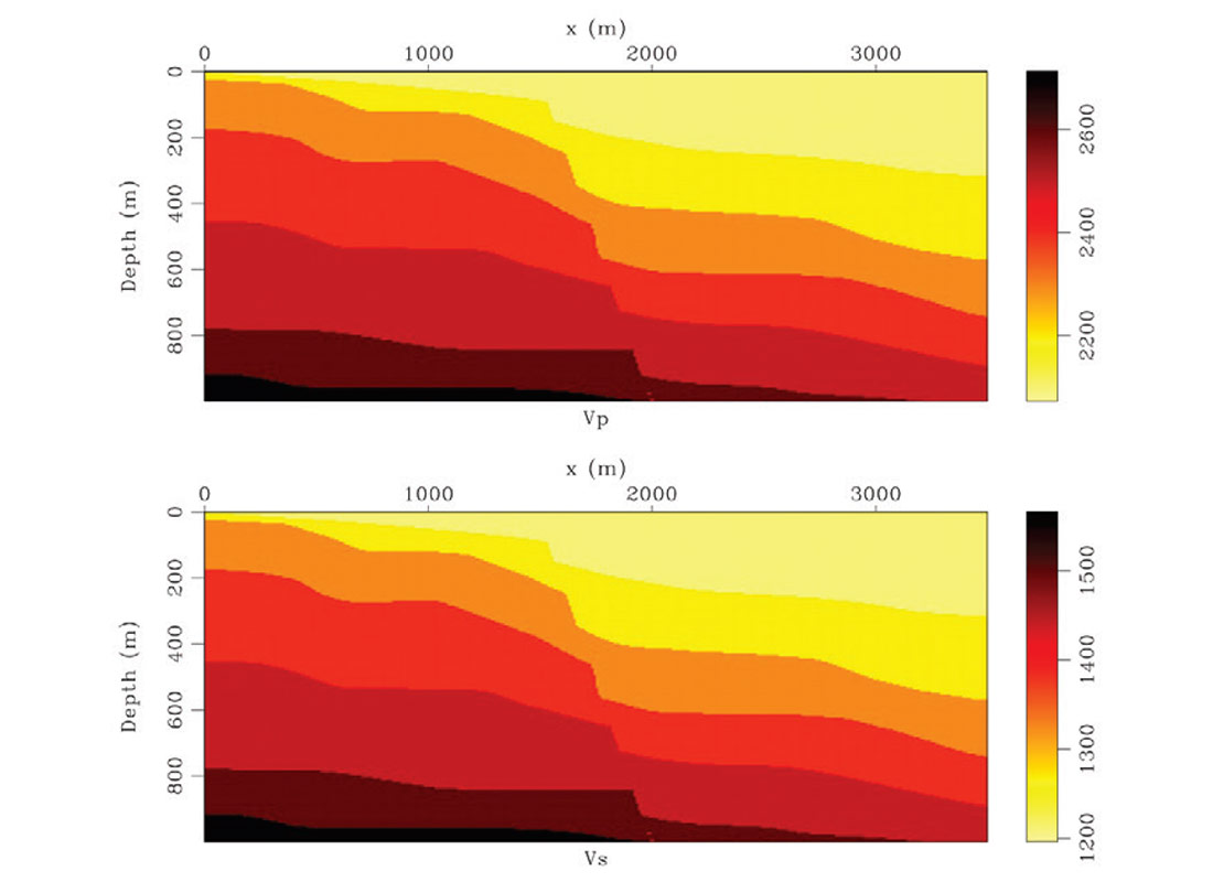
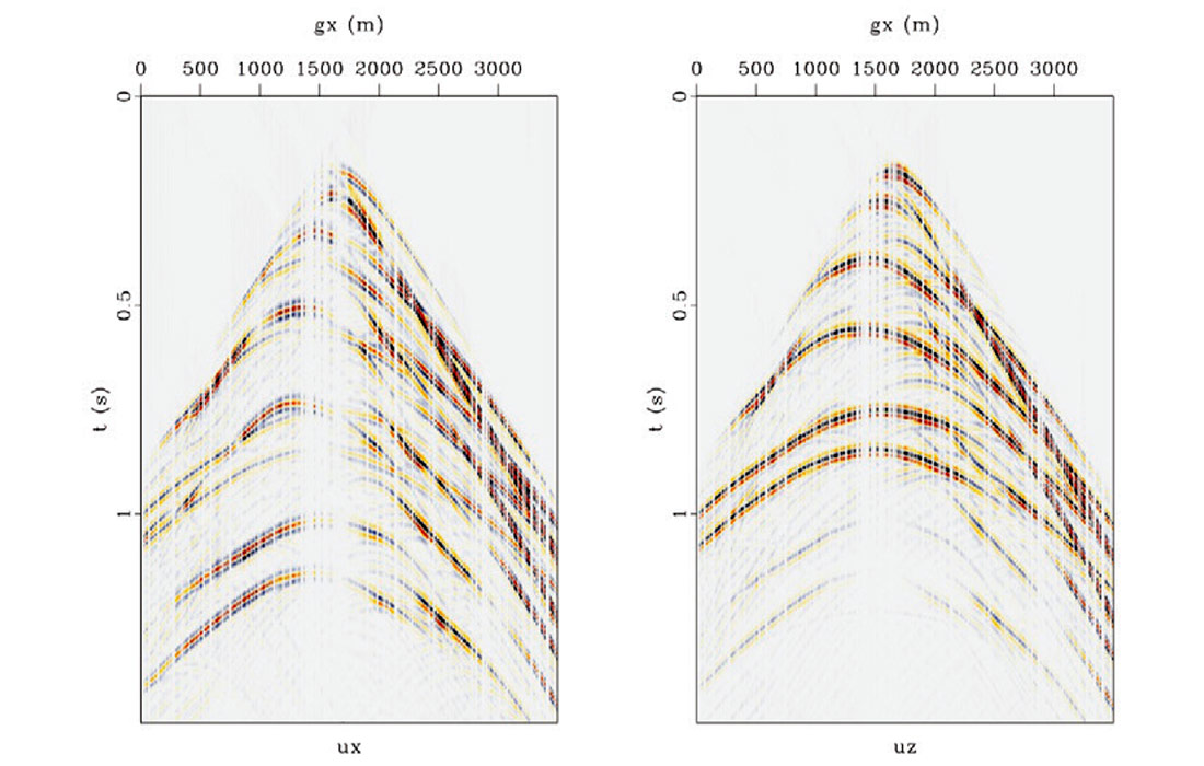
To demonstrate our algorithm we created a model consisting of bedding transected by a normal fault. The P and S wave velocities for this model are shown in Figure 1. We generated 115 two component shot gathers using elastic finite difference modeling using a pressure source with a 40Hz peak frequency Ricker wavelet. A representative shot gather is shown in Figure 2. Notice the mixture of PP and PS wave events between components. We decimated 50% of the receivers randomly to simulate a more realistic acquisition scenario. Under perfect sampling our Helmholtz decomposition operator, H, performs well in decomposing the vector wavefield to P and S potentials. Figure 3 shows the result of migration for a constant opening angle of -42°. Because of the missing data the wavefield separation did not perform well and some cross-talk persists in both images. Figure 4 shows the result of 5 iterations of least squares migration. Clearly the wavefield separation has been improved as the cross-talk artifacts have been reduced. Another improvement comes in the form of resolution. Figure 5 shows the amplitude spectrum for the migrated (blue) and least squares migrated data (red). For both m_pp and m_ps the amplitude have been broadened for low and high frequencies. Figure 6 shows the misfit for 5 iterations of CG. The algorithm required just a few iterations to converge to a satisfactory result.

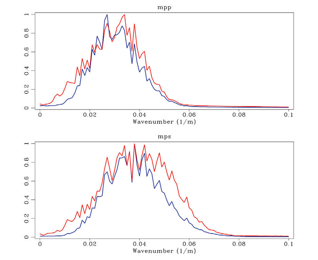
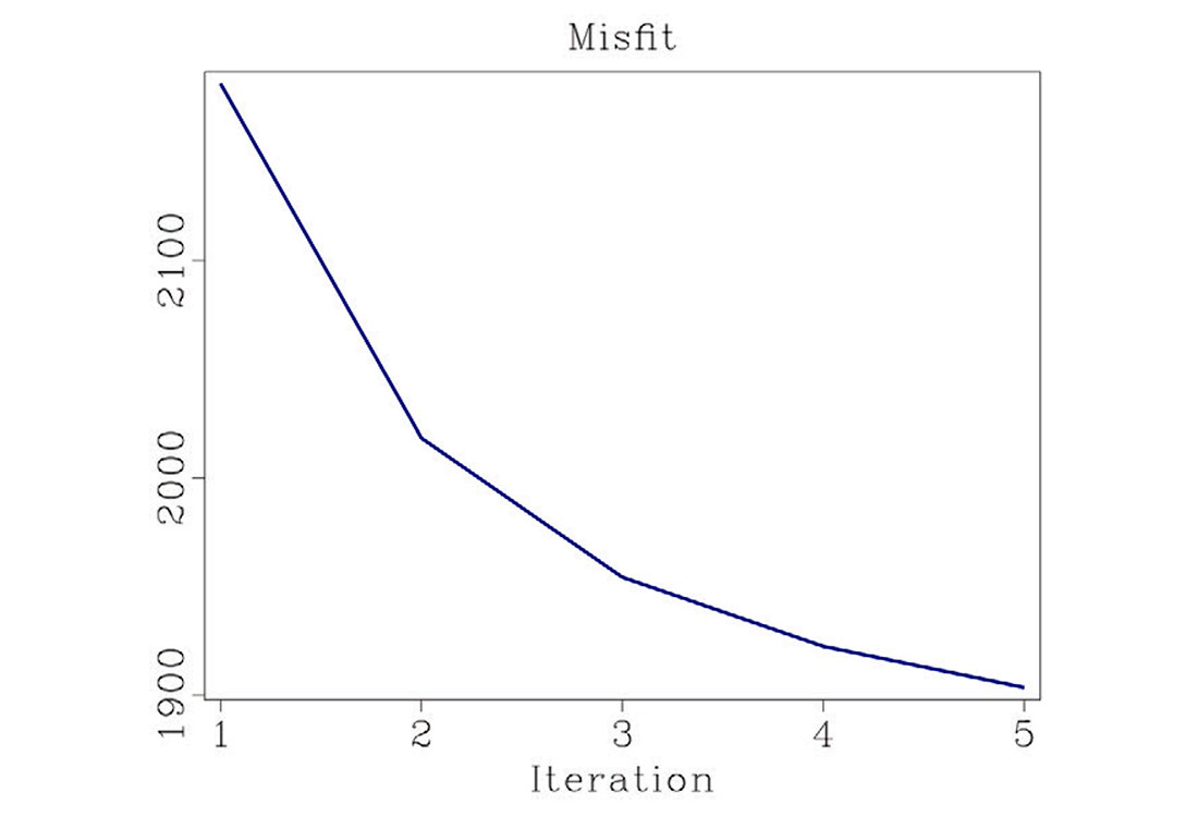
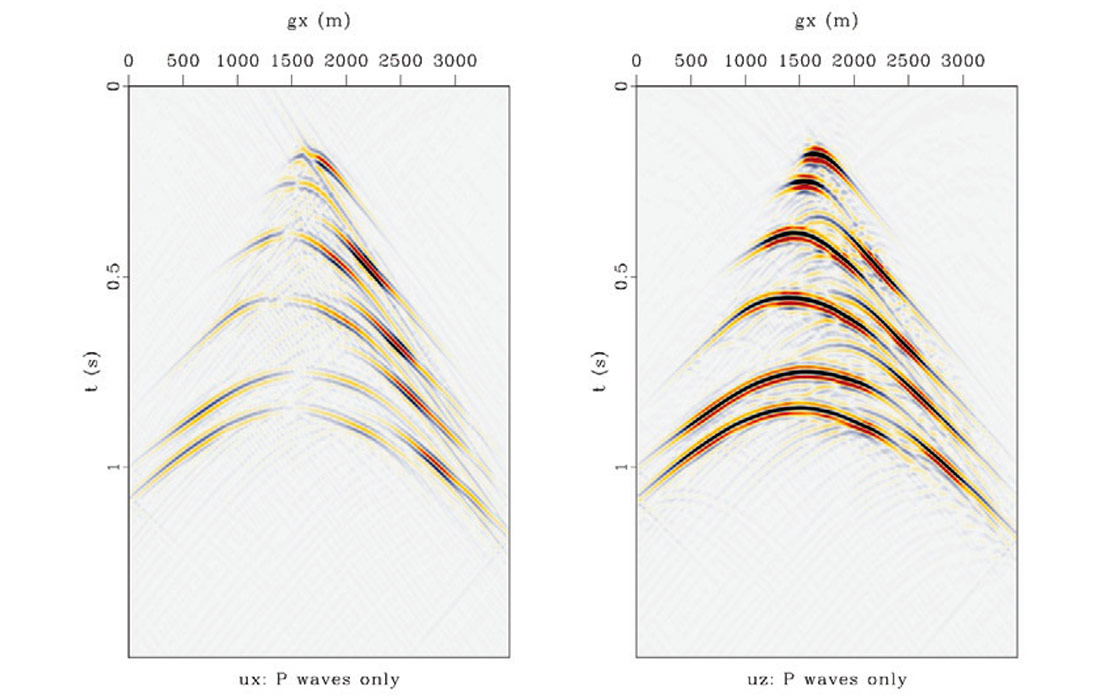
Figure 7 demonstrates two interesting applications of elastic least squares migration: interpolation and wavefield separation. After finding an acceptable image that best fits the data, the forward operator can be applied to predict data:

This prediction can be used for interpolation and denoising of the data. For wavefield separation one of the images mpp or mps can be set to zero allowing for the prediction of P waves on both components (or vice versa). In Figure 7 we see the result of predicting P waves at all trace locations for one shot. This approach can be used to predict entirely new source locations, or as shown in this case, to infill missing receivers for a previously existing source.

Conclusions

Least squares migration algorithms attempt to fit recorded data with predictions generated from a migrated image. By improving the accuracy of the migration operator to include elastic wave propagation we expect to improve the ability of least squares migration to fit seismic amplitudes. Our example demonstrates that least squares migration can improve the resolution of PP and PS images. The algorithm can also be used for data reconstruction and wavefield separation.

Acknowledgements

We thank the sponsors of the Signal Analysis and Imaging Group for their continued support, and Westgrid for computational resources. The figures in this article were generated using the open source software Madagascar.