Introduction
The target audience of this article is the geoscientist who desires to learn more about seismic inversion and its limitations. The content is especially relevant to those using seismic inversion to help build static reservoir models for field development and/or estimate probabilities for presence of hydrocarbons. The viewpoint and experience base of the authors (at least the first author) is that of a consumer of seismic inversion as opposed to a provider of inversion software or services or a researcher in inversion. We have assumed that the reader has some knowledge of AVO and statistics. Our treatment of the probabilistic versus deterministic topic is not detailed – we intentionally focus on concepts instead of theory and equations. If we are successful in engaging the reader in this topic, the reader will have many follow-up questions.
In the title of this article, we have used the terms deterministic and probabilistic to describe two different approaches to seismic inversion. While the reader may not be familiar with these terms used in the context of inversion, the geoscientists that interpret seismic data, generate structure maps and estimate hydrocarbon volumes of prospects and fields will be familiar with deterministic and probabilistic reserve estimates. The input variables in those reserve estimates – porosity, water saturation, gross rock volume and recovery factor – frequently have a range of values and probabilistic reserve estimates attempt to deal with these uncertainties by representing field reserves as a distribution characterized by the P10, P90 and mean reserve size. Contrasted with the probabilistic approach is the deterministic field reserve method where a geophysicist estimates a single reserve volume. The deterministic method will commonly be used to give a ‘best estimate’ or ‘most likely’ case, but it can also be used to generate ‘high-side’ and ‘low-side’ hydrocarbon volumes. Probabilistic and deterministic reserve estimates – and the associated concepts about uncertainty – are a very good analogue for dealing with the uncertainties inherent in seismic inversion. This article shows how seismic inversion is non-unique. A deterministic seismic inversion is any inversion that outputs just ONE of many different acceptable inversion solutions. An alternative inversion approach is to search for ALL of the acceptable inversions (or more realistically, the statistics that characterize those inversions) which we refer to here as a probabilistic inversion.
Inversion terminology
Before getting into a discussion of inversion and non-uniqueness, it is helpful to define some of the terms we will use here. There will be a more detailed technical discussion of these terms later.
Forward model
Forward model refers to the algorithm used to generate synthetic seismic data. As geophysicists, we have some very complex forward models like a full elastic wave-equation and simple models like the convolutional model. A common forward model used in post-stack inversion consists of calculation of reflection coefficients from an impedance model and convolution of those reflection coefficients with a source wavelet. For pre-stack inversion, the forward model needs to be expanded to include AVO effects – which is usually done by use of Shuey’s equation.
Model-based inversion
A model-based inversion uses a forward model (see above) to calculate synthetic seismic data as part of the inversion algorithm. All of the inversion techniques discussed here – deterministic inversion, probabilistic inversion, stochastic inversion and GLI inversion – here are model-based inversions.
Property models: impedance model, Vp model, Vs model, rhob model
Property models are the input to a forward model. They are also the output of a seismic inversion. For a post-stack inversion the property model is an impedance model. Pre-stack inversions require input (Vp, Vs, and rhob) property models.
Relative and absolute inversion/ Relative and absolute property models
Most inversion algorithms solve for absolute property models (ie absolute impedance for a post-stack inversion) which are comparable to impedances from well log data. Creating relative impedance is one method for dealing with non-unique inversion results. Relative impedance models show – in a relative sense – high and low impedances that correspond to different lithologies, but those relative impedances are not are not comparable to the absolute impedances of well logs. The key difference between relative and absolute impedance is that a relative impedance model is missing the low frequency component (approximately 0-15 Hz) found in an absolute impedances model.
GLI inversion
Generalized linear inversion (GLI) has been and probably still is the most commonly used seismic inversion technique. For each post-stack trace or pre-stack gather inverted, GLI inversion requires that the user supply a single initial estimate of the earth’s property model(s) which is iteratively refined so as to give a synthetic (via the forward model) to match the seismic data being inverted. GLI will output a single impedance model for each trace or gather inverted.
Stochastic inversion
Stochastic inversion uses an alternate process of searching through many different input model but refining none of them. The searching process includes generating a synthetic (via the forward model) and comparing the synthetic to the data being inverted. The models corresponding to a ‘good fit’ between this synthetic and the seismic being inverted are kept as output inversion models. The ‘bad fit’ property models are discarded. The input models are built using distributions of earth property models generated from well data Stochastic inversion usually outputs the average of all the ‘good fit’ property models but it can output just the single best fit property model.
Deterministic inversion
Deterministic inversions will output just one earth property model. GLI inversion is always a deterministic inversion. If stochastic inversion is outputting only the best fit property model it finds, then it is a deterministic inversion.
Probabilistic Inversion
Probabilistic inversion is a term we use here to denote those inversion algorithms that combine stochastic inversion with Bayes’ Theorem1 to give rigorous probabilistic estimates of reservoir properties and pore fluid (brine vs water vs gas). Probabilistic inversion is expensive and difficult to use, but it can solve a long-standing challenge in our industry; how to use seismic attributes in a quantitative manner for risking exploration and development prospects. Probabilistic inversion is an evolving technology, both in a technical and commercial sense.
Geostatistical inversion
Geostatistical inversions are stochastic inversions that use variograms to prepare the input property models. The purpose of those variograms is to ensure that the property models fit expected spatial patterns (i.e. facies models). We will not discuss geostatistical inversion here.
Probabilistic and deterministic inversions have different but overlapping uses. Table 1 attempts to organize a high-level view of where one might best apply deterministic and probabilistic inversions. On the top row of Table 1 are some different applications for seismic inversion. These are: to facilitate interpretation of geology and stratigraphy, as an initial scan for hydrocarbons, calculating the probability of hydrocarbon presence and using inversion to help build a static reservoir model. With the first column, we distinguish between inverting post-stack seismic data for AI and the more complex task of inverting pre-stack data for AI and Vp/Vs (or various other pairs of rock properties). The point of this table is that deterministic inversions are more appropriate for the simpler inversion applications in the upper left, while the more quantitative inversion applications in the lower right are better served by a probabilistic inversion. Other factors that influence the decision to use probabilistic inversion are its requirement for appropriate trend data from well logs (discussed below) and the need for significantly more computer power than that required for deterministic inversion.
| Stratigraphic interpretation | Scan for hydrocarbons | Risk hydrocarbon presence | Build static model | |
|---|---|---|---|---|
| Table 1: Recommended applications for deterministic and probabilistic inversion. | ||||
| Post-stack inversion for AI | Deterministic | Deterministic / Probabilistic | Deterministic | Probabilistic |
| Pre-stack inversion for AI & PR | Deterministic | Deterministic / Probabilistic | Probabilistic | Probabilistic |
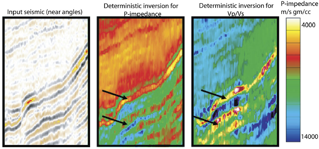
Figure 1 shows a line from a 3D seismic survey and the associated GLI/ deterministic inversion results. This GLI inversion was used to interpret geology/ stratigraphy and to initially highlight the presence of hydrocarbons. One discovery and two delineation wells were drilled based on this inversion. These deterministic results were followed up with probabilistic inversions used to risk the presence of gas in near-by fault blocks, estimate volumes of gas present and to help build static and dynamic reservoir models. We will use this same data set to calculate a probabilistic inversion later in this article. But before we discuss the deterministic and probabilistic inversion of this dataset, we first need to explain how GLI inversion can be nonunique. That requires a bit of background on GLI inversion.
Deterministic/ GLI Inversion
How GLI inversion works
For this explanation of GLI inversion, we will simplify things by assuming the forward model and input data are post-stack and the property model being inverted for is thus an impedance model2. The GLI impedance model is ‘parameterized’ using blocky impedance layers. For each blocky layer in the model, there are two parameters; one that describes the layer impedance and one that describes the layer thickness. Both the input usersupplied initial impedance model and output final impedance model are parameterized in this manner. The objective of the inversion algorithm described below is to iteratively update these impedance parameters so that a synthetic trace made from this impedance model matches the input seismic trace being inverted.
Figure 2 illustrates how the deterministic GLI inversion algorithm works. This is an iterative algorithm that proceeds in the clockwise direction as per Figure 2. In the upper right is an input seismic trace to be inverted. In the upper left is a user-supplied initial impedance model. The user also needs to supply a source wavelet3. The input impedance model is an estimate of the true earth impedance model and may have significant errors. A forward modeling algorithm generates a synthetic trace from this impedance model and source wavelet. For a simple inversion example, the forward modeling algorithm just calculates reflections coefficients from the impedance estimate and then convolves those reflection coefficients with the source wavelet. Other more sophisticated forward models could include multiples and/or prestack AVO effects.
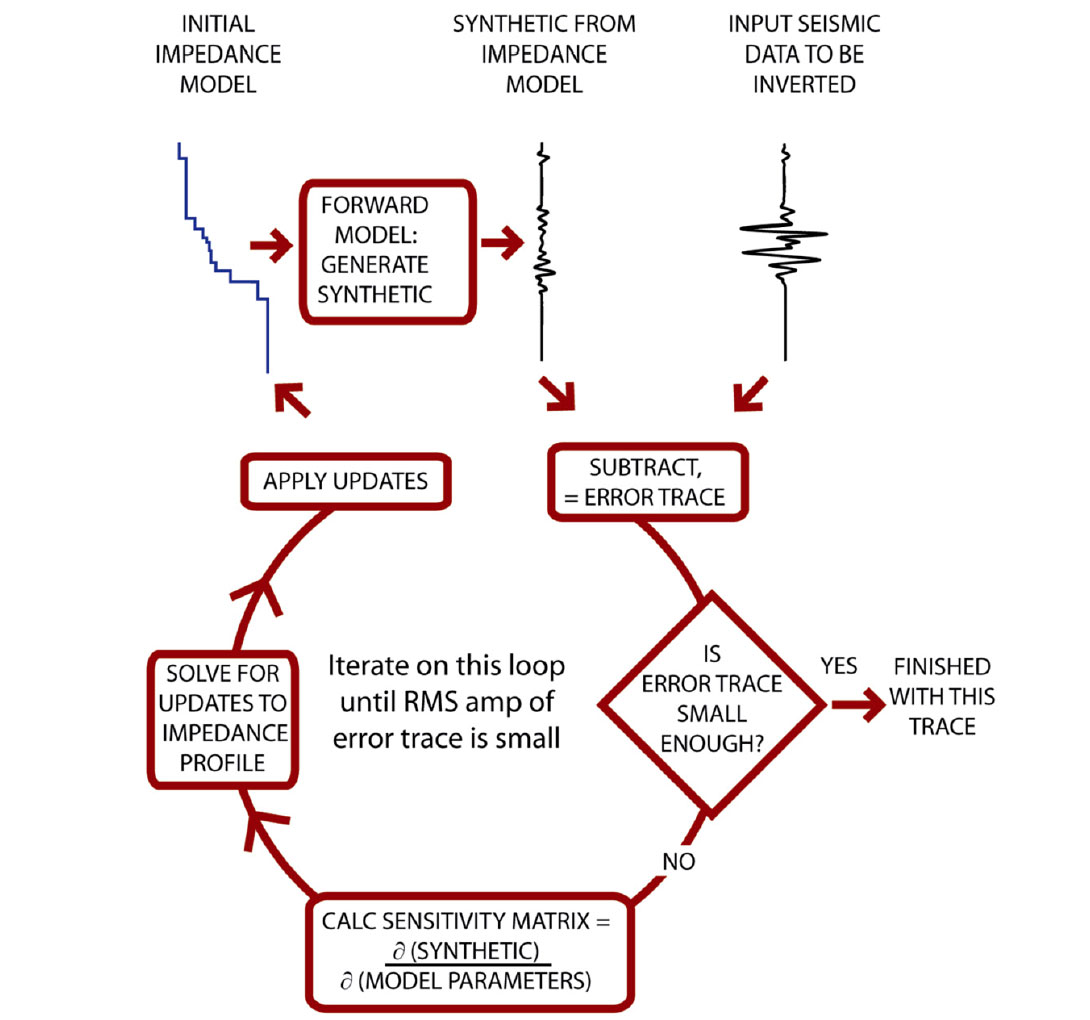
The next step is to subtract the synthetic trace from the real trace. The result of this subtraction is called the ‘error trace’. At the diamond shaped box, the algorithm checks for exit conditions from this iterative loop. The main exit condition is the RMS amplitude of the error trace. If this RMS amplitude is low enough the algorithm exits from the loop. Other possible exit conditions are that ‘enough’ iterations have occurred (usually 5 to 10) or that convergence has stopped – that is the RMS error is not getting smaller with successive iteration.
If an exit condition has not been met, the inversion loop proceeds to the ‘calculate sensitivity matrix’ step which explores the relationship between each impedance model parameter and the current synthetic trace. In mathematical terms, this step calculates the partial derivatives of the current synthetic with respect to each impedance model parameter (thicknesses and impedance values of each blocky layer in the model). Each partial derivative is a seismic trace or vector. The collection of these partial derivative vectors constitutes the partial derivative matrix or sensitivity matrix which has m rows and n columns, where m is the number of samples in the input seismic trace being inverted and n is the number of parameters in the impedance model.
The next step calculates corrections or updates to the current impedance model using the above error trace and the sensitivity matrix. For the mathematically inclined, these updates come from the truncated (linearized) Taylor-series approximation of the forward model. This is rewritten as:

where:
I = the unknown vector of parameters that describe the real earth’s impedance profile, IG = the user supplied ‘initial guess’ for I that will be iteratively refined in the inversion, F = the forward model algorithm,

(I – IG) = the vector of impedance model updates to be solved for. Once (I-IG) is obtained, the desired result is
I = IG + (I-IG).
Usually, an exact solution to this equation does not exist, so a least squared error technique is used to solve for the impedance model updates term. Furthermore, since the above equation is a truncated Taylor series expansion (i.e. an approximation), the above equation needs to be applied iteratively.
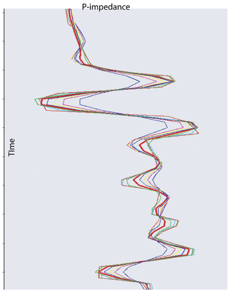
Each pass through the inversion loop ends with adding the above impedance model updates to the current impedance model. Figure 3 shows how each successive iteration through this loop will update the last iteration’s impedance model in a manner that (hopefully) converges on a solution where the error trace is all zeros. At that point, the inversion algorithm will move onto the next input trace to be inverted and continue in this manner until the entire seismic line or volume is inverted.
Discussion of frequency content and uniqueness
Following is a discussion of frequency content and uniqueness explained in the context of GLI inversion, but these non-uniqueness issues are also true for any one single inversion model output from stochastic inversion. This is true because both GLI and stochastic inversion have a mismatch between the frequency content of the property model and the seismic data being inverted.
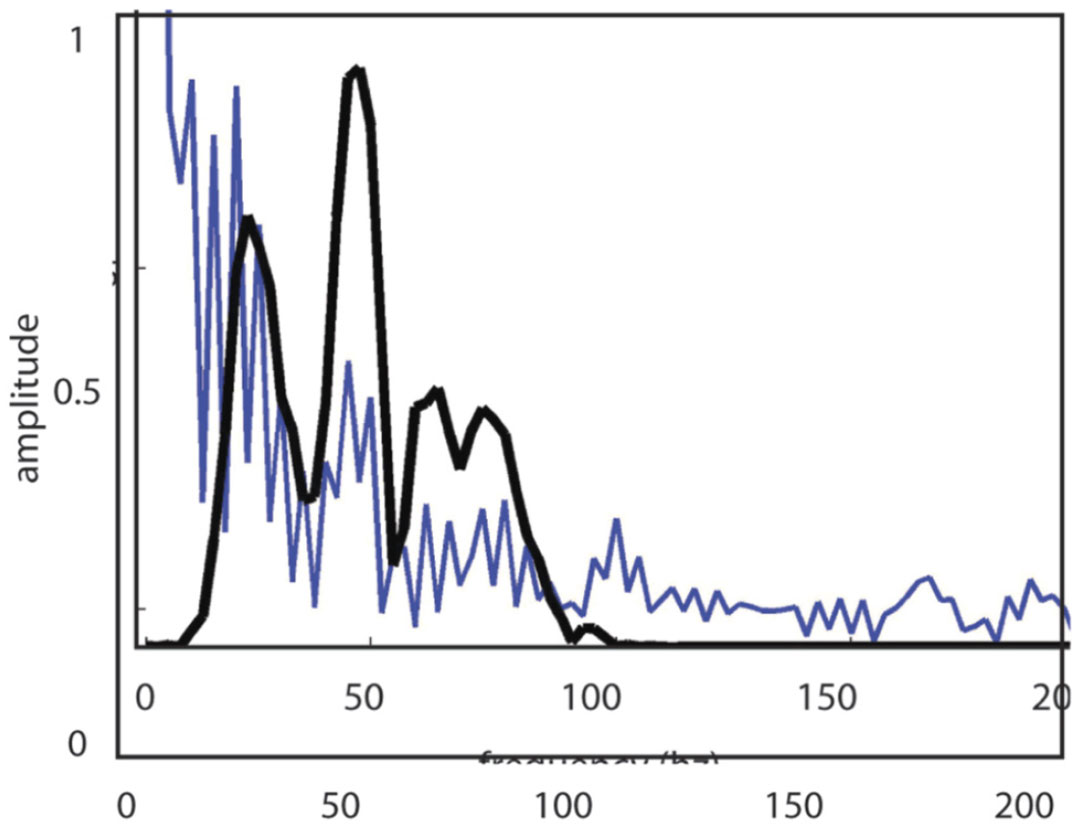
The astute observer may notice that in GLI inversion, the output impedance model appears to have frequency content that is not found in the input seismic trace. In Figure 4, we compare the frequency spectra of input trace and the resultant output inversion model. Clearly, the output impedance model has frequency content below and above that found in the input seismic data. Where did this ‘extra’ frequency content come from? Is the information content of these frequencies reliable? One insight to these ‘extra’ frequencies comes from Figure 2 which shows that the impedance model updates are calculated from real and synthetic seismic data which has limited band-pass, while the impedance model has a much wider band-pass. Most importantly, the higher-than-seismic frequencies and the lower-than-seismic frequencies are filtered out before the ‘calculate sensitivity matrix’ and ‘solve for updates’ steps.
High frequency issues
The higher-than-seismic frequencies in the output impedance model are imposed upon that model by the assumption that the earth’s impedance can be described using blocky impedance. The blocky model assumption contains the high frequencies – not the input data. This is the core assumption of GLI inversion and it is not always valid. Figure 5 shows some reservoirs with impedance models can be described with a blocky model assumption, as well as the coarsening upwards or fining upwards sands that can not be described with blocky layers.
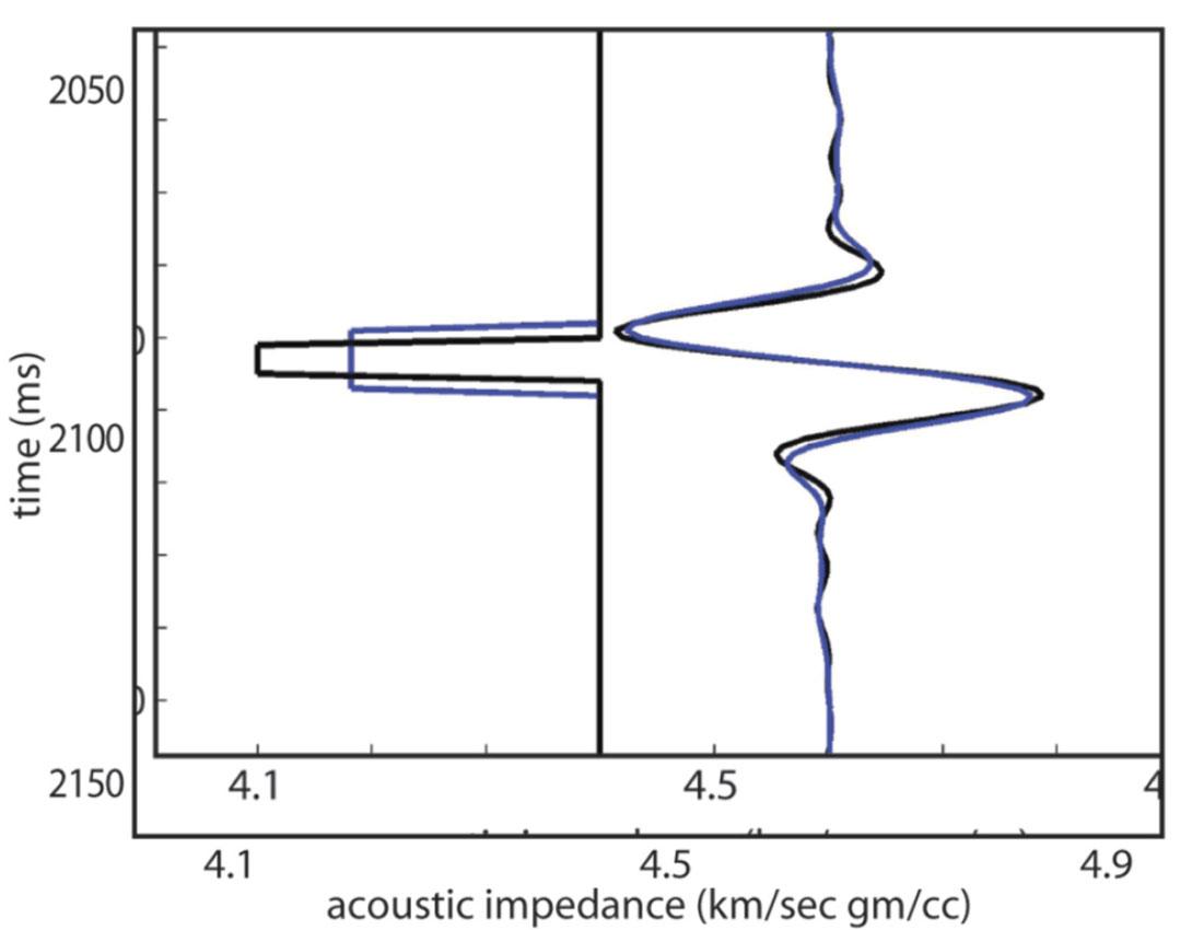
Even if one assumes the earth can be described accurately with the blocky layer assumption, there is the issue of uniqueness for inversion of thin reservoirs (thinner than the seismic tuning thickness). For any reservoir thinner than the tuning thickness, there are an infinite number of reservoir thickness & impedance combinations that give the same seismic amplitude. This is illustrated in Figure 6 which shows two impedance models – both of which are thinner than the tuning thickness – that have very similar synthetic seismograms. For reservoirs thinner than the tuning thickness, GLI and stochastic inversions can not resolve this thickness-impedance uniqueness problem. What combination of impedance and thickness will model-based inversion output for such thin reservoirs? A GLI inversion will output the first impedance and thickness combination it finds that meets the exit conditions in Figure 2. A stochastic inversion should, in theory, output all of the acceptable property models (or a representative distribution of those models).
Low frequency issues
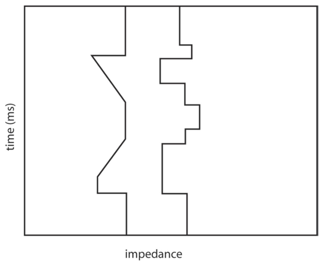
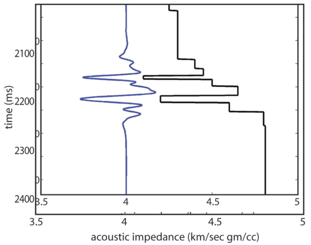
As with the higher-than-seismic frequencies, the lower-thanseismic frequencies in the output impedance model are problematic. As mentioned above, the iterative inversion loop of Figure 2 filters out the lower-than-seismic frequencies before calculating the sensitivity matrix and impedance model updates. Figure 7 illustrates the ambiguity that results from filtering these low frequencies. The two impedance models of this figure differ in their low-frequency content (and their absolute impedance values) but have the same synthetic seismic trace. Clearly, the model-based seismic inversion of this trace is non-unique.
Where do the lower-than-seismic frequencies in the output impedance model come from? The simple answer is that the low frequencies largely come from the user-supplied initial impedance model. The GLI impedance model updates will occasionally change those low frequencies, but it is difficult to predict when this will happen or how significant the change to low frequencies will be. The low frequencies in the output impedance model are dominated by the low frequencies in the user-supplied initial impedance model which is normally interpolated and extrapolated from well control. That interpolation/ extrapolation step can miss important low frequency anomalies not sampled by the well control – for example over-pressure cells and the associated velocity reductions.
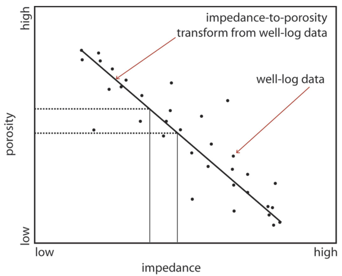
What is the practical impact of non-unique low frequencies in the impedance model output by deterministic inversion? If an inversion is being used to interpret stratigraphic boundaries and geometries, then the impact is not significant. If the inversion is being used to scan for gas, then this low frequency non-uniqueness could cause problems but only if the interpretation of gas is based on the absolute impedance value (as opposed to an interpretation based on changes impedance or relative impedance). And if the impedance inversion is being using to calculate porosity (perhaps for a static model) then those porosity values will be non-unique as shown in Figure 8.
Above we have discussed possible impedance errors at high and low frequencies. There are two possible ways to deal with these errors: the relative impedance approach and the probabilistic impedance approach.
Relative Inversion
The relative impedance approach recognizes that while a GLI inversion has problems with the lower-than-seismic and higherthan- seismic frequencies, the impedance inversion is reliable and unique over the seismic bandwidth – and can be filtered back to the seismic band-pass. Figure 9 shows the relative impedance model that corresponds to the absolute impedance models in Figure 7. The relative impedance ‘solution’ ensures that the GLI impedance inversion results are not be misused. However, the relative inversion approach is perhaps overly conservative and certainly does not help those who are trying to use seismic impedance inversion to build a reservoir static model that has thin blocky reservoir intervals populated with absolute porosity values.
Probabilistic/stochastic inversion
The relative inversion solution discussed above is one way of dealing with non-unique inversion results. Relative inversion essentially filters out all of the non-unique – and potentially misleading – information. This filtering may be a bit drastic as the blocky layer assumption for thin reservoirs is frequently correct, as is the lower-than-seismic portion of the input initial model. An alternate way of dealing these non-unique solutions is stochastic or probabilistic inversion which attempts to find ALL of the acceptable earth impedance models (or the statistics that represents all acceptable impedance models). The motivation for doing many different inversions on the same input trace is the recognition that a single model-based inversion result has nonunique high and low frequency content (discussed above). The high/ low frequency content of an inversion solution is influenced by the high/ low frequency of the initial impedance model – so the input models for probabilistic/ stochastic inversion are chosen to sample the range of range of possible input models.
The major components of probabilistic inversion are:
- Review/interpret well data. Extract property trends (for Vp, Vs and rhob) and their standard deviation
- Stochastically sample above trends searching for property models that match (via the forward model) the input seismic data being inverted.
- Use Bayes’ Theorem to calculate probabilities
We explain each of these three aspects of probabilistic inversion in more detail below.
Well data trend analysis
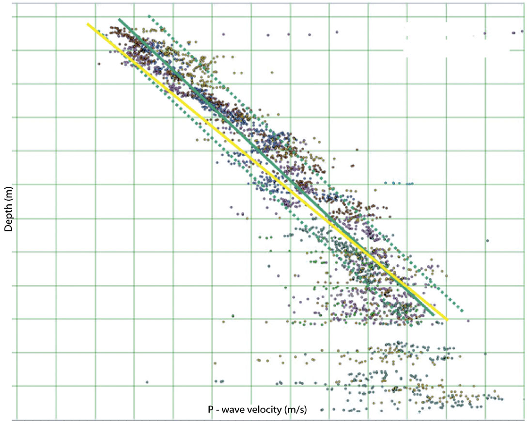
Probabilistic/stochastic inversion needs information about the distribution of properties (Vp, Vs, rhob) in the input models. These distributions are generated prior to the inversion using local well log data. This is a somewhat interpretive step called trend analysis. Well data trend analysis starts with selecting relevant wells (we usually need a minimum of three to five wells) and manually interpreting/ picking a lithology flag. The lithology flag just indicates which intervals should be in the sand trend analysis and which intervals should be in the shale trend. Figure 10 shows an example output Vp trend analysis for sand and shale. (This figure is from a location different from Figures 1, 11, 12 and 13. This well trend data set was chosen to illustrate how sand and shale trends converge with depth and how pressure impacts velocity.) Note that the average Vp trend and its standard deviation are defined in this analysis. These trends are defined as a function of depth and apply to an inversion over any depth interval. Once the depth coordinate of the inversion is specified, a distribution of Vp (mean plus standard deviation) can be extracted from this trend. A similar process is done for Vs and rhob, however, Vs and rhob trends are developed as a function of Vp, not as a function of depth. This allows linking the stochastically simulated values of Vs and rhob to the simulated value of Vp. Trend analysis can be time consuming and rather interpretive, but results are a regional database that can be applied to inversion of many different seismic datasets in the same basin.
Generate and evaluate the input models
A stochastic inversion will generate many different input (Vp, Vs, rhob) models from the above distributions, generate synthetic seismic data from each model, and keep the models with a ‘good fit’ (i.e. low RMS (data – synthetic trace)) with the input seismic data being inverted. The input models are frequently called prior models or priors and the good fit output models are called posterior models. For a stochastic inversion to output statistically correct models, it must sample the above input property distributions in a fair manner. As an example of an ‘unfair’ process, consider property models that are generated only using the slow velocities in the above input well data distributions. The ‘good fit’ models output from that stochastic inversion will have correspondingly slow velocities and will not accurately represent reality. The more sophisticated stochastic inversions use a process called Markov Chain Monte Carlo (MCMC) sampling to ensure fair sampling of input distributions.
The exact details of how a stochastic inversion builds prior models impacts the inversion’s the ease of use and reliability of the results. To help the reader understand this important step we describe the model building process used by just one probabilistic inversion: Delivery4 (Gunning and Glinsky, 2004). Delivery requires the user to specify a generic layer input model that includes all of the possible lithologic layers for the seismic data being inverted. The user must also supply a structural interpretation from which to ‘hang’ this generic model. The generic model needs to include the sealing shale units above and below the reservoir and all sands, shale breaks and hard streaks within the reservoir interval. Delivery can/will give erroneous results if this generic input model can not describe the real earth. An example of this would be if the real earth has a significant shale break not included in the input model. There will typically be three to a dozen layers in a generic input model. Reservoir layers have an additional parameter that indicates pore fluid (brine/ low saturation gas/ gas/ oil). Initially, the properties (Vp, Vs, rhob and thickness) of each layer in this generic input model layer are not assigned. A MCMC process is used to sample well data trends, assign layer properties to create hundreds of prior models. Those prior models will included brine or pay in the reservoir layers. (more detail about this in the section on Bayes’ Theorem below). Gassman-Biot fluid substitution is used to change the Vp, Vs and rhob of reservoir layers as the pore fluid changes.
Bayes’ Theorem and probability estimates
Bayes’ Theorem is frequently written as:

Where P(a|b) is shorthand for ‘probability of event a being true given b’, and P(a) is ‘probability of a’. P(a) in the numerator is usually called a prior probability. It is much easier to explain Bayes’ Theorem if we rewrite it in terms of gas probabilities for a prospect that has an observed seismic attribute as below. The seismic attribute is AVO fluid factor in this example, but we could use any other seismic attributes instead of fluid factor.

Where P(gas| ff=0.25) means the probability of finding gas given our prospect has an fluid factor=0.25. For this first simple example, we assume this prospect can be modeled by a single blocky sand between 2 shales where the properties of the shale and wet sand (Vp, Vs and rhob) have distributions that are known from local well data. Gas sand properties are calculated using Gassman-Biot fluid substitution. Well control also supplies a distribution of expected reservoir thicknesses. To generate the term P(ff=0.25| gas) in the numerator, we stochastically simulate many gas charged reservoir models, generate a pre-stack synthetic from each model and calculate the AVO fluid factor for the top of the reservoir for each model. The red curve in Figure 11a shows the probability density function (PDF) of calculated fluid factors for these gas simulations. This curve is generated assuming gas is present (i.e. P(ff| gas)) so the area under the curve equals 1. In this figure we have also generated and displayed a PDF for fluid factor assuming that the reservoir sand is wet (blue curve).
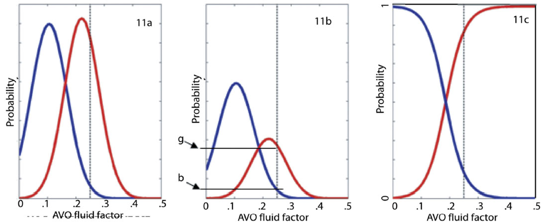
Figure 11b shows the wet and gas fluid factor PDFs again, but this time we have scaled the P(ff|gas) and P(ff|brine) curves using the prior information that – for this one example – the probability of gas is 1/3 and the probability of brine is 2/3. The scaled gas curve is equivalent to P(ff|gas) x P(gas) in the numerator of Bayes’ Theorem. In this simple example we excluded the possibility of oil filled reservoir.
The denominator in Bayes’ Theorem refers to the probability of observing a fluid factor=0.25 and needs to includes both true positives (gas is present) and false positives (brine is present). Using the values g and b denoted on the vertical axis in Figure 11b, the denominator in Bayes’ Theorem is then g + b. And the probability of finding gas for a fluid factor= 0.25 is:

Figure 11c shows probability of gas calculated for all fluid factors values.
The above example of Bayes’ Theorem was worked through using a single seismic attribute (fluid factor). This workflow is becoming more common in companies that wish to quantify hydrocarbon risk using attributes, but instead of using a single attribute (like stack amplitude or fluid factor) many companies are using 2-dimensional PDFs made with inverted AI and inverted PR or some other set of AVO attributes.
In the above example, we have ‘inverted’ seismic data for gas probability and explained Bayes’ Theorem when the observed seismic data is a single number (fluid factor=0.25). This work flow works quite well when ‘inverting’ a map of fluid factors (or other seismic attributes) – but we have assumed a simple single blocky sand reservoir. A more sophisticated probabilistic inversion will need to invert a full seismic trace instead of an attribute. For that case, Bayes’ Theorem is implemented thus: some of the input (prior) property models have brine in the reservoir and some have hydrocarbons. The exact ratio of hydrocarbon models to brine models in the prior models is determined by the prior estimates of gas- i.e. P(gas) in the numerator of Bayes’ Theorem. The stochastic inversion will generate synthetics and keep only those which prior models fit the seismic data; these models are the posterior models. The revised Bayesian probability of gas is the ratio of number posterior hydrocarbon models to the sum of number of posterior hydrocarbon models + number of posterior brine models.
For both the trace-based and map-based probabilistic inversion, P(gas) is a required user input that specifies a prior estimate for presence of gas. This prior usually comes from traditional prospect risking workflows where P(gas) = P(reservoir) x P(seal) x P(hydrocarbon charge) x P(structure).
A comparison of deterministic and probabilistic results
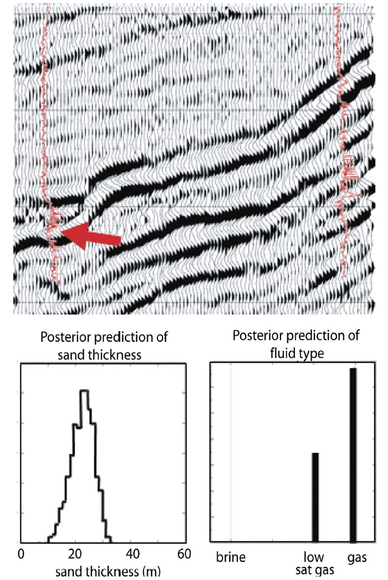
Figures 12 and 13 show typical results from a probabilistic inversion. The input seismic data to this inversion was the same set of 3D gathers as for the deterministic inversion in Figure 1. For the probabilistic inversion, the generic input property model had 5 layers covering ~100ms of data (plus the ‘half-spaces’ above and below). The required well log trends were developed using eight wells within 30km. There are two wells on this line; the information from them was input to the trend analysis, but the exact log data was not known to the probabilistic inversion. Figure 12 shows the probabilistic inversion’s posterior model distributions for sand thickness and reservoir fluid. These distributions are for just one layer at one gather. Similar distributions also exist (but are not shown) for porosity, sand/shale ratio, P-impedance and Vp/Vs for each model layer at each CMP5. These inversion solutions (the posterior solutions) consist of approximately 2000 property models that provide a good fit to the seismic data for each input gather in a 3D survey. This is a very large amount of data that is best displayed and interpreted using cumulative probability statistics ( P10, P50 and P90) as in done Figure 136.
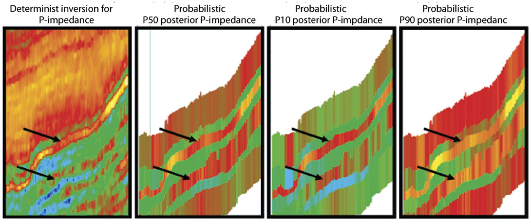
In Figure 13 we compare the deterministic inversion P-impedance results of Figure 1 to the probabilistic P-impedance (P10 P50 P90 displays). There is a common user expectation that the P50 probabilistic result should be equal to the deterministic result. In our opinion, the deterministic and P50 probabilistic inversion results will always be equal only if both are filtered back to the seismic band-pass and if the probabilistic results have a normal distribution. In Figure 13 we can see that the deterministic and P50 probabilistic results are equal for the upper gas reservoir (arrows denote gas reservoirs), but not for the lower gas reservoir. What are causing these differences for the lower reservoir? Possible answers are:
- The probabilistic inversion is restricted to 5 layers, while this deterministic inversion algorithm has much finer layer sampling.
- The non-unique low frequencies are treated differently in the two inversion algorithms. The deterministic inversion uses a low frequency model that is interpolated between well control. The probabilistic inversion does not know about this spatially variable low frequency model; it only knows about an average P-impedance and its standard deviation.
We think the major driver behind the different inversion results for the lower reservoir is that the deterministic inversion performed a narrow (and incomplete?) search for solutions. Its search started with a user-supplied low frequency trend from a nearby well and stopped with the first solution it found. The probabilistic inversion searched for all solutions suggested from trend data from eight wells.
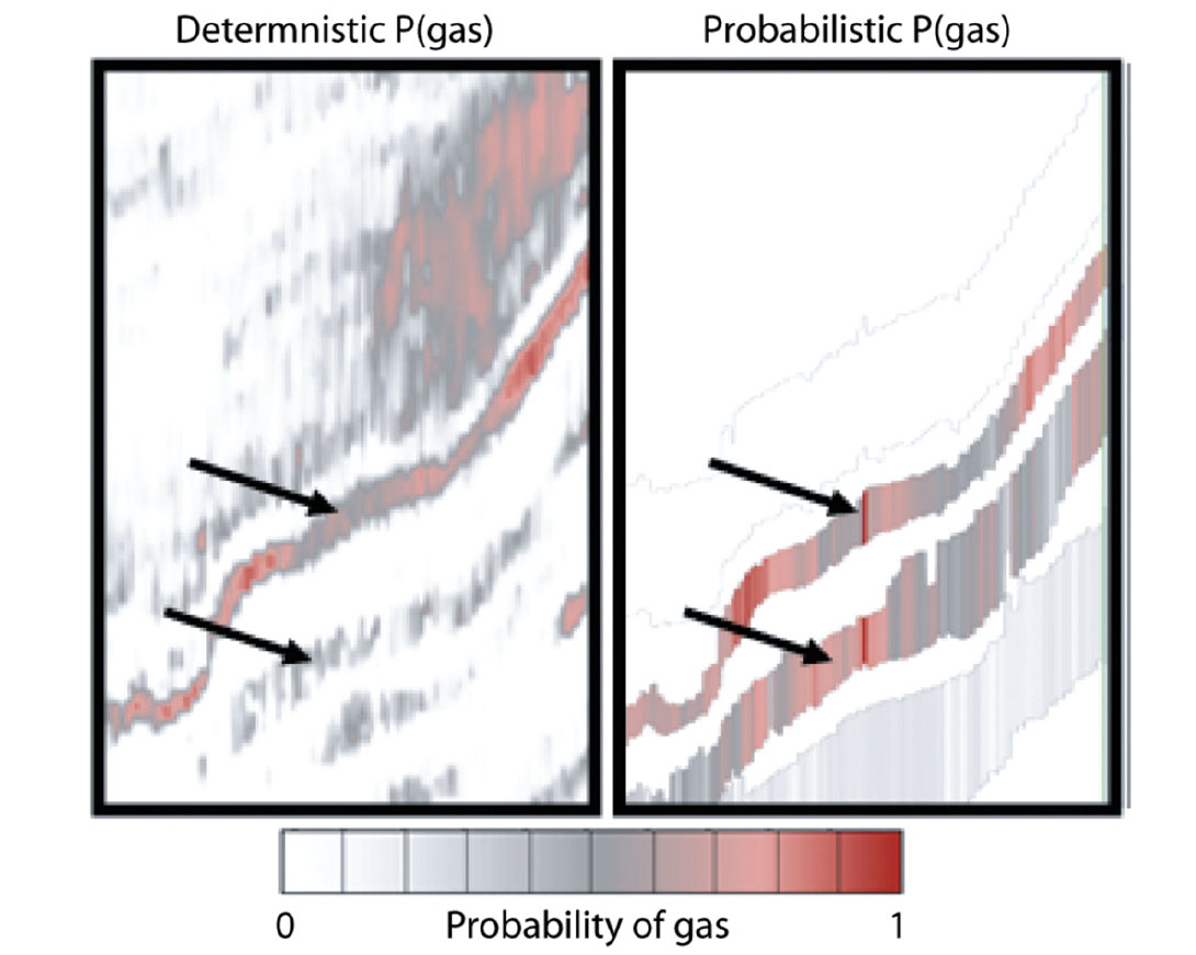
Probabilities for gas can also be calculated from deterministic inversion via a workflow that uses Bayesian logic to compare inversion results to well data much like the section on Bayes’ Theorem above. Figure 14 shows the probabilistic inversion’s probability of gas and compares it to a similar prediction from the deterministic inversion. Again, these results are the same for the upper reservoir and different for the lower reservoir – and again we think the differences are expected due to the different treatment of the low frequency model.
Summary and Conclusions
There are many ambiguities inherent in inverting seismic reflection data to log data. A deterministic model-based inversion will output just one earth impedance model that ‘fits’ the seismic data being inverted, and the user of that deterministic inversion has a risk of being proven wrong by the drill bit. With a probabilistic model-based inversion, all acceptable earth impedance models are output.
The section above hints at some rather interpretive aspects regarding probabilistic inversion and low frequencies: what weight should be applied to existing prior information about low frequencies? Should the nearest well have higher weight than trends established by a population of wells? We note that this is a problem that geostatistics is well posed to answer. We also note the technique of using migration velocities to constrain low frequency trends. Migration velocities might supply the required low frequency velocities, or – due to the fact that imaging velocities are not the same as true velocity – the migration velocities may be ‘misinformation’.
The promise of a probabilistic model-based inversion is not that it resolves the inherent ambiguities, but instead it quantifies them. The accuracy of that quantification is linked to applicability of the input trend data. Assuming the trend data is applicable, the quantification of unknowns can be quite helpful when making investment decisions on expensive oil and gas wells.

Acknowledgements
The authors would like to thank Santos, Ltd for supporting the ongoing effort to study this topic and for permission to publish this article.
Related Reading


Join the Conversation
Interested in starting, or contributing to a conversation about an article or issue of the RECORDER? Join our CSEG LinkedIn Group.
Share This Article