Geophysical Well Logs from a Shallow Test Well and Automatic Determination of Formation Velocities from Full-Waveform Sonic Logs

Abstract

Shallow VSP and geophysical well logging surveys were undertaken in a 127 m-deep well located at the Rothney Astrophysical Observatory site near Priddis, Alberta. The well was drilled through interbedded sands and shales of the Paskapoo Formation. A suite of geophysical well logs (including natural gamma-ray, normal resistivity, focusedbeam resistivity, density, neutron-neutron, caliper, temperature, and SP) was acquired in the open hole immediately after drilling. After PVC casing was inserted into the well and grouted to the formation rocks, we obtained natural gammaray and full-waveform sonic logs. The logs were useful for delineating the sandstone and shale beds, and for providing hydrogeological information at the well site.

To analyze full-waveform sonic data, we formulated procedures for trace alignment, noise reduction, and automatic time picking of first arrivals. The resulting time shifts and first-break times were used with the known geometry of the full-waveform sonic tool to determine P-wave velocities of the rock formations around the well.

Introduction

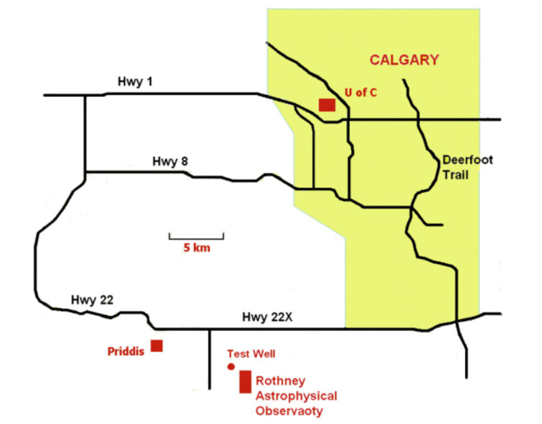
The Paskapoo Formation in the Foothills region of Alberta is the groundwater source for over 100,000 water wells. Characterizing the hydrogeology of the formation, which consists of Tertiary-age shales and sandstones, is a major undertaking by government and university institutions (Grasby et al., 2006; Natural Resources Canada, 2007). As a localized contribution to the overall investigation, we conducted geophysical well-logging in a shallow test well drilled into the Paskapoo Formation for the University of Calgary. The well is located near Priddis, Alberta at the site of the Rothney Astrophysical Observatory, about 50 km from the U of C campus (Figure 1). For the Geoscience Department, the test well is an important addition to its teaching and research infrastructure, as it provides convenient opportunities for demonstrating and evaluating downhole field techniques in geophysics and hydrogeology.

The test well

Over a three-day period in August, 2007, Aaron Water Well Drilling Company of Dewinton, Alberta, used an air-rotary rig to drill the well with an open-hole diameter of 156 mm. The static water level was 30 m below ground surface after the drilling ended at the target depth of 137 m. To protect against caving of the overburden into the well bore, the driller inserted steel casing to a depth of 5.5 m with a projection of 0.61 m above ground level. To prevent long-term collapse of the well, a quarter-inch-thick (6.35 mm), 4.0-inch- ID (102 mm) PVC casing was inserted to a depth of 127 m. There was a one-day delay between the end of drilling and the insertion of the PVC casing, so that open-hole geophysical logging could be done. During this delay, rock detritus washed out of fracture zones fell to the well bottom and caused the loss of about 10 m of well depth.

The well was intended to provide a research and teaching facility and not to produce water for domestic or commercial uses. As such, there is no well screen, and the PVC casing is closed off at the bottom and not perforated. Following standard procedure in Alberta for the completion of shallow water wells, the casing was sealed to the rock with a combination of bentonite grout and bentonite pellets to prevent vertical groundwater flow.

Interpretation of open-hole well logs

After the target depth of 137 m was reached, but before the well was cased, Roke Oil Enterprises Limited was retained to provide a suite of open-hole geophysical logs. These logs are presented on Figures 2 and 3. The 16-inch normal resistivity and natural gamma-ray logs have variations that follow closely the beds of shales and sandstones within the Paskapoo formation. Shale layers coincide with low resistivity values and high gamma-ray activity; sandstone beds coincide with higher resistivities and lower gamma-ray activity. Other openhole logs vary with lithology in similar fashion. High values on the neutron-neutron log and focusedbeam resistivity log can be correlated with sandstone, while low values can be correlated with shale. The density and caliper logs indicate significant fracturing in the upper 60 m of the well.

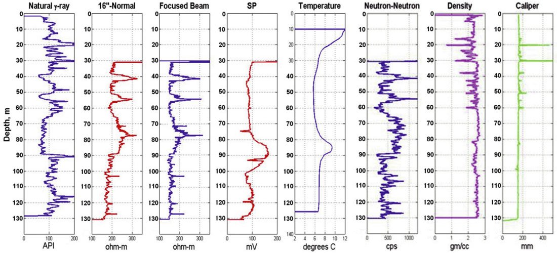
The SP (spontaneous potential) and temperature logs are relatively flat with broad maxima occurring at depths between 80 m and 90 m. The sharp peaks on the SP log are probably measurement errors. The SP log from the test well is unusual. Normally, SP logs follow variations in lithology, with SP lows associated with shales and SP highs associated with sandstones. Steps and linear gradients on a temperature log often indicate water inflow and outflow, and flow between permeable zones. The broad maximum near 85 m on the temperature log is consistent with a zone of weak groundwater inflow near the base of the large sandstone unit that extends from approximately 63 m to 90 m in depth. The temperature log was taken within hours after drilling was completed, so that thermal equilibrium had not been reached.

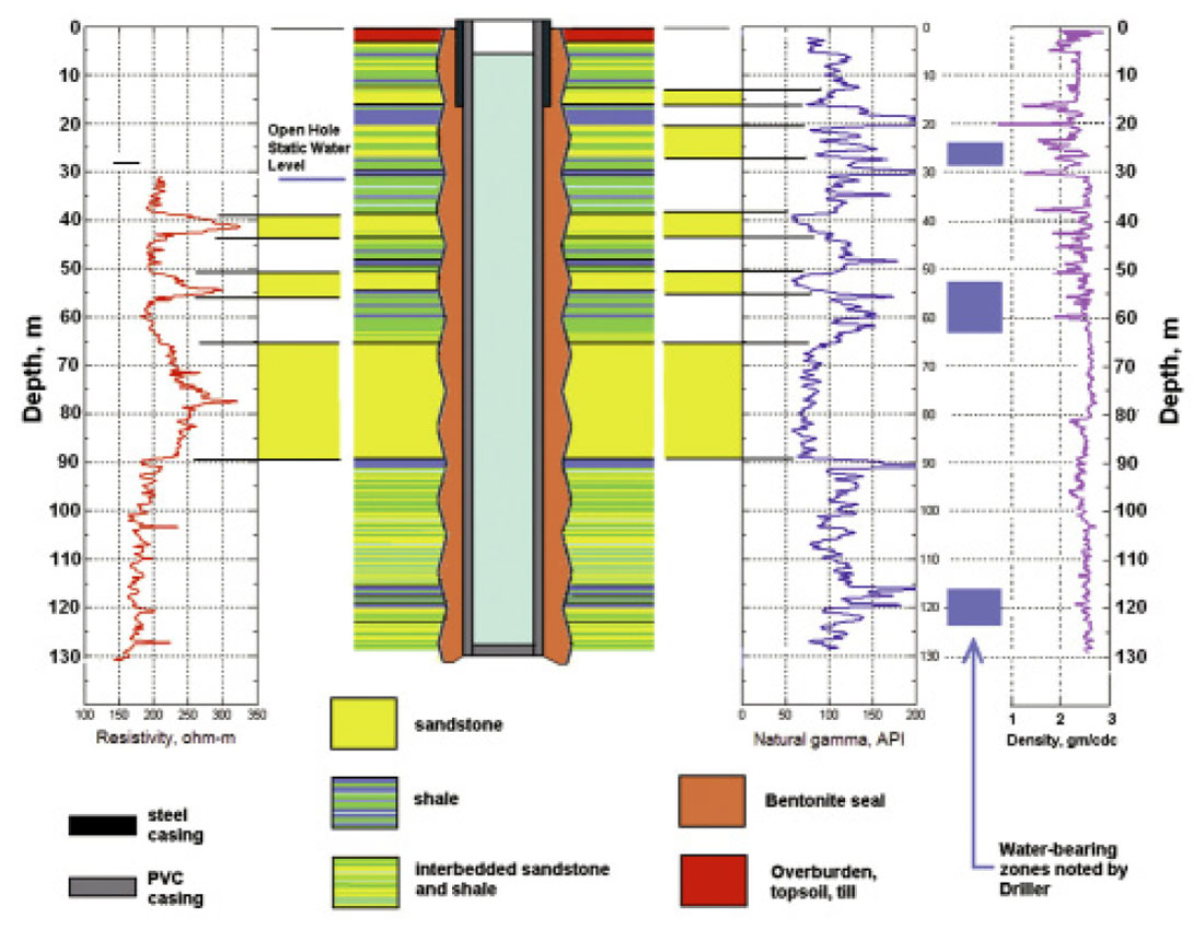
Figure 3 shows the construction details of the well and the geological materials it encountered. The lithology log is an interpretation of cuttings described by the driller and the resistivity and natural gamma-ray logs shown on the figure (Miong, 2008). Fracturing in the upper 60 m of the well is indicated by the sharp decreases on the density log. Water-bearing zones, reported by the driller at depths of 24 to 28 m, 52 to 63 m, and 116 to 122 m, are shown in blue. We can relate these zones to sandstoneshale interfaces interpreted from the resistivity and gamma-ray logs, and to fractures indicated by the caliper and density logs. The near-surface aquifer at 24 to 28 m flowed at a rate of 15 gallons/minute. The driller measured the total dissolved solids (TDS) in this water to be about 300 ppm, declaring this to indicate excellent groundwater quality. The large fracture at 20 m, and fractures in the thin beds of sandstone and shale at depths between 22 m and 29 m, are likely the source for the fastflowing water.

The open-hole static water level at 30 m coincides with the large fracture shown by the caliper log at the same depth.

Listening to the well after drilling had stopped but before casing was installed, we could hear the sound of falling water. The static level and the sound of falling water suggest that the fractured sandstones above 30 m are a source of water, but the fracture at 30 m is a sink. This was confirmed during sealing of the well with bentonite grout. The grout is a slurry of water and bentonite that is pumped from the surface to fill the gap between the casing and the rock formation through a flexible plastic tube called a tremmie pipe. The slurry filled the gap effectively from the well bottom up to a depth of 30 m. But then a large volume was pumped into the gap without the grout level ever rising above 30 m. In the end, the driller poured solid bentonite pellets into the gap to complete sealing the top 30 m of the well.

Cased-hole well logs

The Department of Geoscience at the University of Calgary held its 2007 Geophysical Field School at the Geophysical Test Site near the Rothney Observatory. One of the School’s activities was well-logging using a Mount Sopris Instruments Matrix II geophysical logging system in the test well. The system hardware includes natural gamma-ray, single-point resistance, spontaneous potential, and full-waveform sonic tools. Because the well was completed with PVC casing, we used only the natural gamma-ray tool and the full-waveform sonic (FWS) tool. To provide coupling to the rock for full-waveform sonic logging, the casing was filled from the surface with water. The PVC casing is made up of 20 ft (6.1 m) sections threaded together, and slow leakage takes place through the threads. At the time of the field school, the water level inside the well was about 6 m below ground level.

Natural gamma-ray logs

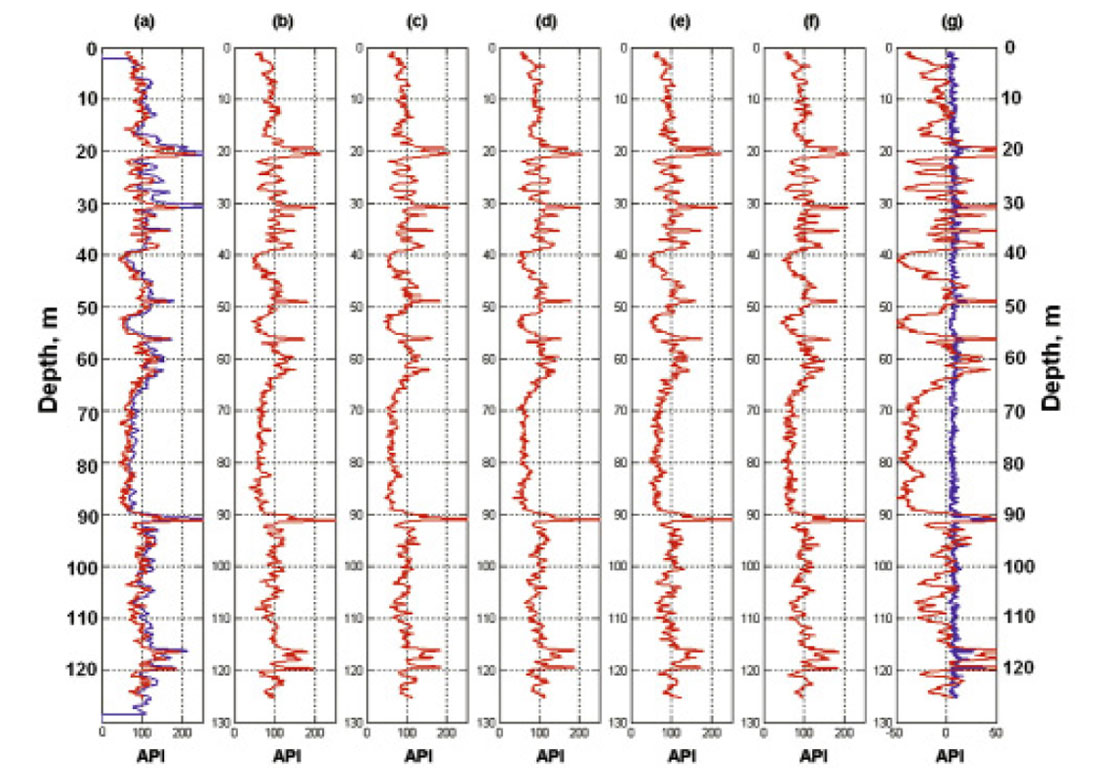
Over the two-week period of the field school, multiple gamma-ray logs were acquired in the cased well. Figure 4 displays six of the gamma-ray logs to indicate how well the results repeat. The blue plot on Figure 4(a) is the gamma-ray log obtained before the well was cased. The open-hole and casedhole gamma-ray logs are almost identical; the only effect of the PCV casing is to decrease slightly the number of gamma rays reaching the detector. On Figure 4(g), the red profile is the average of the six cased-hole gammaray logs minus a constant 100 API units; the blue profile shows the standard deviation of the six logs. The standard deviation values are about 4 to 8 API units, or about 3 to 10 per cent of the average values. The small mismatches between individual logs are due to differences in logging speeds and in eccentric positioning of the gamma-ray tool in the well.

Full-waveform sonic logs

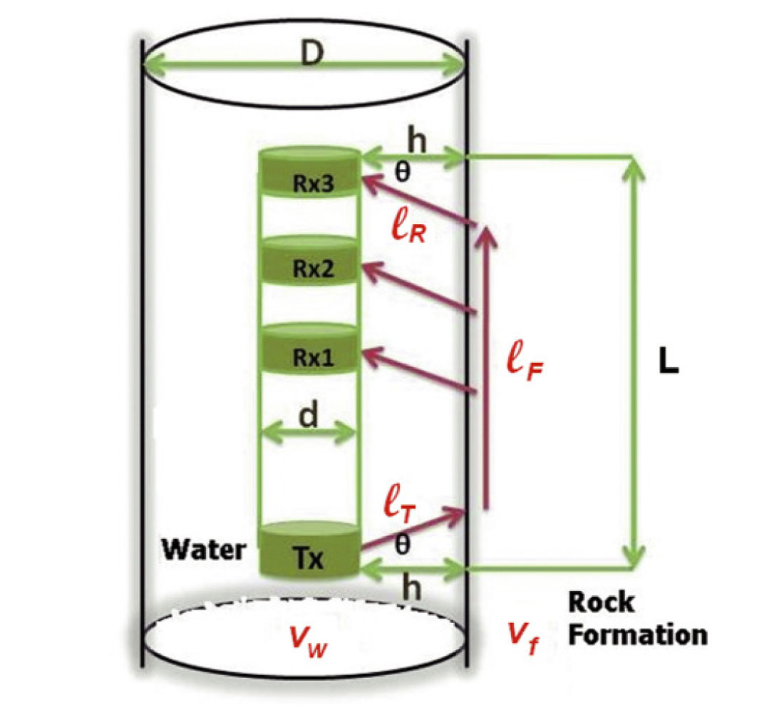
The FWS tool, shown on Figure 5, consists of a stainless steel housing for downhole electronics, a piezoelectric source, and an array of three piezoelectric receivers. The transmitter is located near the bottom of the tool. The receivers (Rx1, Rx2, and Rx3) are located 0.914 m, 1.22 m, and 1.52 m above the transmitter. The tool is about 2.5 m long and has an OD of about 38 mm. During surveying, the tool was centralized in the well bore, and seismograms were acquired with the tool moving either up or down. The transmitter was configured as a monopole for P-wave logging and driven by a pulse with dominant frequency of about 15 kHz. The usual logging speed was 3 to 5 m/s. For each of the three receivers, we recorded seismograms with 525 digital points and 4 μsec sampling at depth intervals of 0.1 m.

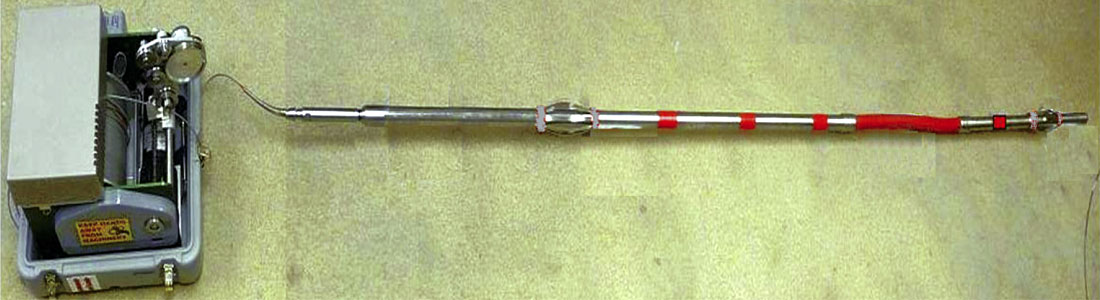
Figure 6(a) displays the raw traces for the Rx1 receiver. The first arrivals are very weak and difficult to see. Because of the low signal-to-noise ratio, picking reliable first-break times on the unprocessed seismograms is very difficult. Figure 6(b) displays the FWS traces after applying an Ormsby bandpass filter (corner frequencies at 10-16-50-80 kHz) and automatic gain control (AGC). The first arrivals are visually much clearer, and it is possible to pick the first-break times manually.

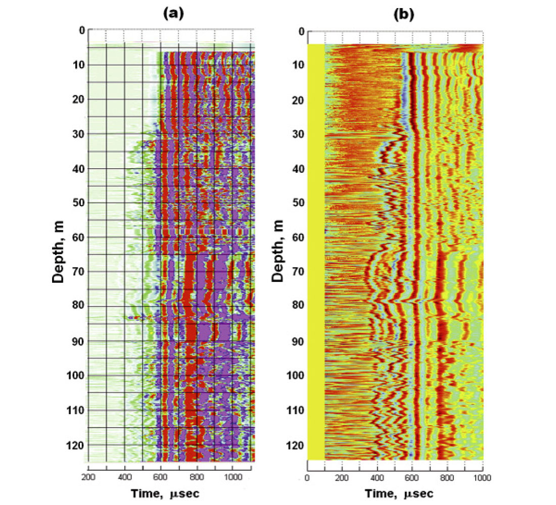
Figure 7 displays two sets of FWS logs recorded on two different days. After filtering and AGC, we see good repeatability for the logs, and first arrivals are clearly visible at most depths for all three receivers. At depths above the water table at 30 m, first arrivals through the rock formation appear to be lost in noise even with AGC. Poor signal amplitudes also occur at a few deeper zones where there is poor coupling between the formation rocks and the well casing, possibly due to washouts or caveins in the well bore behind the casing.

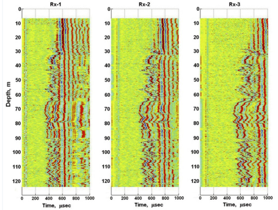
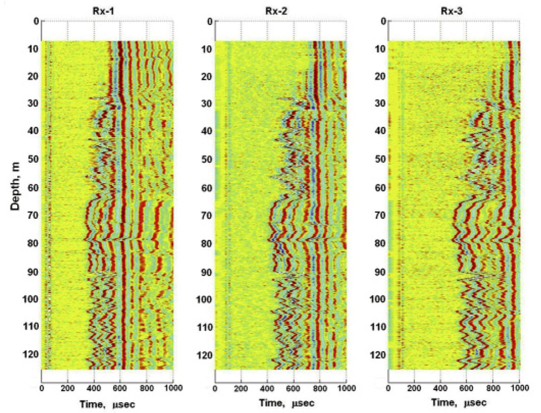
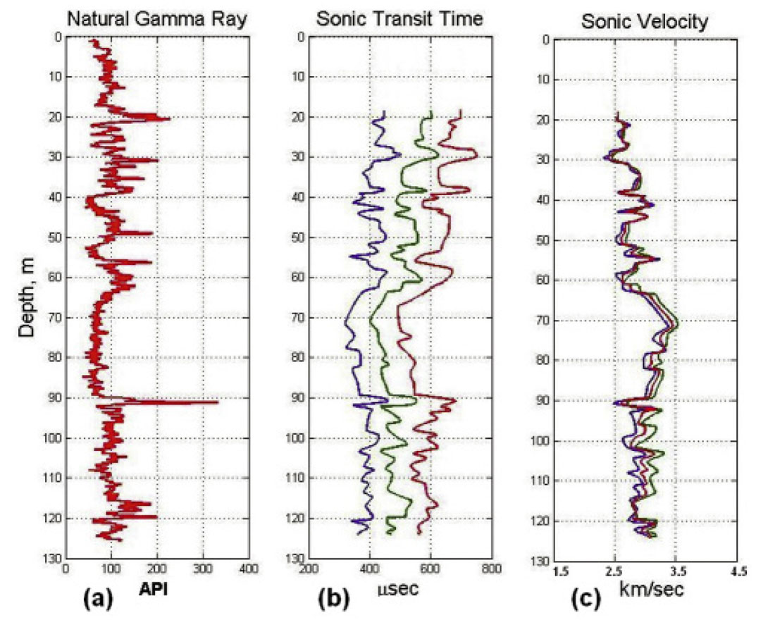
Figure 8(b) shows the first-break times picked manually for the three FWS receivers at depths below 30 m, and the corresponding P-wave velocities. The velocity values were determined from the first-arrival times using the refraction analysis described below. Comparing the velocity profiles on Figure 8(c) with the natural gamma-ray log plotted on Figure 8(a), we see that the lower velocities (2.5 to 2.6 km/s) coincide with high gamma-ray activity associated with shales. Higher velocities (3.0 to 3.6 km/s) coincide with low gamma-ray activity associated with sandstone.

Automatic time-picking

Manual picking of first arrivals on FWS logs is not practical on a regular basis, since a typical FWS log consists of thousands to tens of thousands of seismograms. Automatic schemes for picking first arrival times are essential for such large datasets. Several alternative schemes have been described by Willis and Toksoz (1983), Coppens (1985), and Boschetti et al. (1996). We have developed an automatic picking method based on a modified energy ratio attribute that is suitable for seismograms that have been preprocessed with noise reduction algorithms.

Noise reduction

Both random noise (caused by the tool rubbing against the casing as it moves) and source-generated tube waves are present on the FWS log traces. Both types of noise interfere with automatic first-arrival time picking. This interference must be removed or minimized. Since slow, high-amplitude tube waves have velocities less than that of the water in the well, we can eliminate their influence by muting the seismograms for times following the expected water-wave arrival time. This was done by applying a tapered window whose leading edge is set at a time corresponding to the fastest expected rock velocity (say, 6.5 km/s), and whose trailing edge is set at the time of the waterwave arrival. After windowing, we decreased the influence of random noise by finding a phase-aligned average of several adjacent input traces.

The depth increments between receiver channels and recording stations are small, and the piezoelectric source is highly repeatable. Consequently, the first-arrival waveforms of adjacent seismograms (after filtering, AGC, and windowing) are quite similar, and so averaging them to reduce noise is a valid procedure. Noise reduction by averaging results in significant improvement in first-arrival picking accuracy. We use a minimum variance principle to do trace averaging on the windowed seismograms. Averaging is done in two ways. The first, which we call channel averaging, is applied to the traces from the three receivers at a given transmitter depth. The second, which we call depth averaging, is applied to the traces for a fixed receiver (Rx1, Rx2, or Rx3) at several adjacent transmitter depths.

Minimum variance averaging technique

At a fixed transmitter depth, first arrivals detected by the three receiver channels are delayed systematically as the receiver distance from the transmitter increases. The delays are related to the formation velocity, and we use this fact to do channel averaging of the raw FWS seismograms. After bandpass filtering and AGC, we keep the Rx3(t) seismogram fixed in time and systematically shift the Rx2(t) and Rx1(t) traces forward by times of Δt and 2Δt. We then window, normalize, and average the three traces. Next, we find the difference or error between the average trace and the shifted and unshifted traces. The sum of the squared errors over all the time indices is referred to as the variance νar(Δt). The variance is calculated for many values of Δt, and will be a minimum when the windowed waveforms from the three channels are in phase. The average trace m(t) and the variance νar(Δt) as functions of time shift Δt are given by the following formulae:

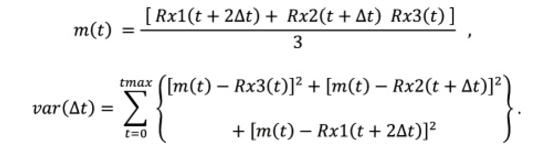
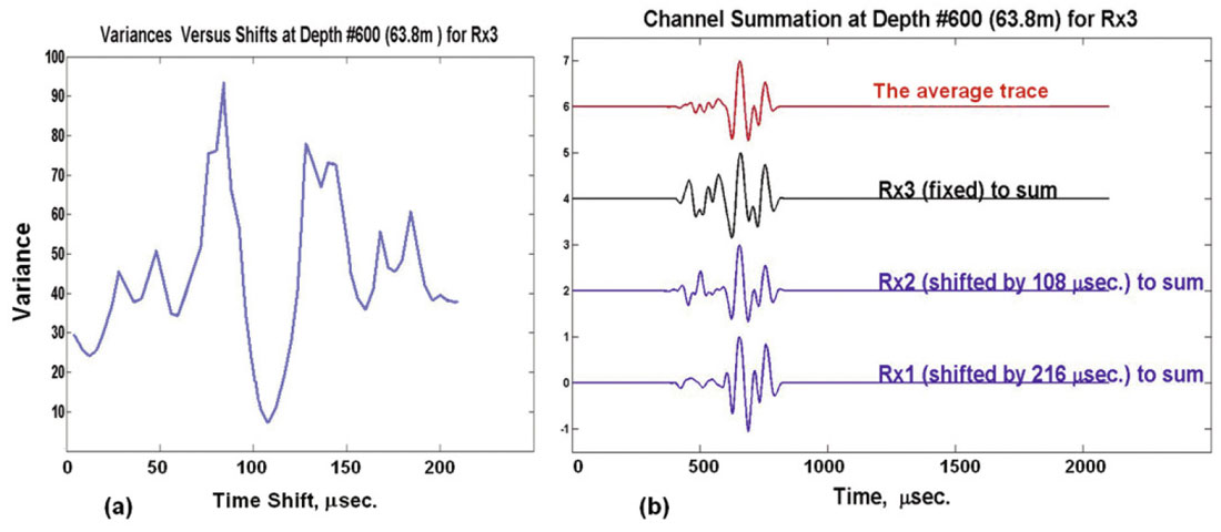
Figure 9(a) is a plot of variance versus time shift Δt using the windowed receiver traces shown on Figure 9(b). The value of Δt that gives the minimum variance value aligns the three input seismograms. When the input traces are thus aligned and added, the random noise preceding the first arrival on the averaged sum trace m(t), plotted in red on Figure 9(b), is much reduced. The average trace m(t) is then used to replace the unshifted input trace Rx3(t) for automatic first-arrival picking.

Similarly, random noise on seismograms can be reduced by averaging over depth. For a given receiver channel, windowed traces immediately above and below and centered about a reference depth are time shifted and added to get an average trace (the trace at the reference depth is not shifted, and time shifts for the traces above and below can differ in both sign and magnitude). The average trace giving the minimum variance with respect to the input traces is used to replace the reference trace for firstarrival picking. The depth-averaged trace is usually calculated with input traces from 3, 5, 7, 9, or 11 depths.

Trace alignment using the minimum variance method closely resembles procedures used for finding and applying trim statics in surface reflection processing. For aligning a few FWS input traces, the minimum variance method is simpler and, we believe, more suitable than the commonly used cross-correlation and semblance techniques (Sheriff, 2002).

Time-picking and modified energy ratios

Our automatic first-arrival picking algorithm is based on a modified energy ratio attribute. On a windowed digitized seismogram, we define:

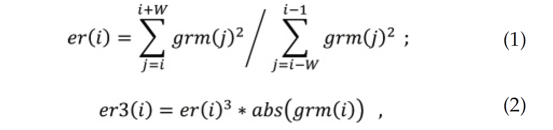
where grm(j) is the seismogram value at time index j, er3(i) is the modified energy ratio at time index i, and W is the length of the energy evaluation windows preceding and following the test point i. The energy window length W is an adjustable parameter, but it must be long enough to include 2 or 3 cycles of the dominant frequency. The first-arrival time pick occurs when er3(i) is a maximum, and this can be determined quite accurately by computer when interference from random noise and tube waves are minimized. Figure 10 is an example of the procedure. The input raw seismic trace shown in dark blue on Figure 10(a) is windowed by the red trace. The leading edge of the window is located at a time equal to the source-receiver distance divided by the maximum velocity expected for rocks, say, 6.5 km/s. The trailing edge is set at a time slightly less than the arrival time expected for a tube wave or a water wave. The windowed input trace is shown on Figure 10(b). The modified energy ratio calculated for the windowed input trace is plotted in green on Figure 10(c), and it can be seen that the first arrival time corresponds very closely to the peak of the modified energy ratio. The peak on the modified energy ratio trace stands out even more if a channel-averaged trace is the input.

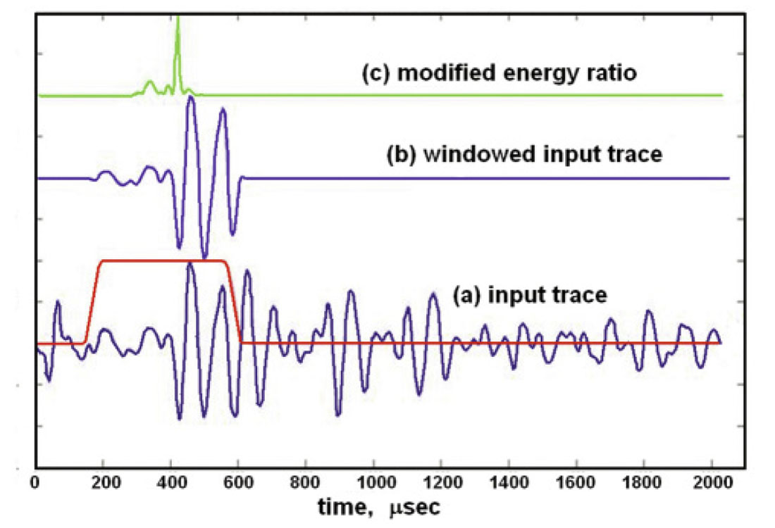
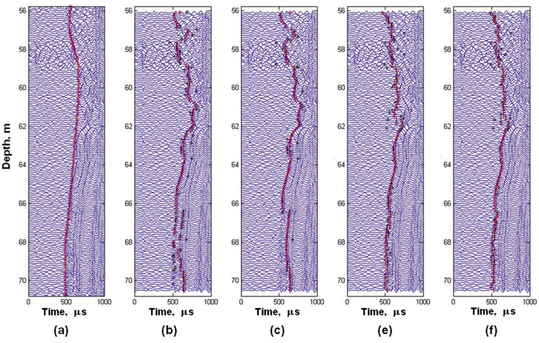
Figure 11 displays automatic picks from both low-noise and high-noise FWS seismograms from the test well. Automatic timepicking using the modified energy ratio attribute works quite well when the signal-to-noise ratios are high. However, where the first arrivals are weak even after noise reduction, the time picks can be erratic. On the same figure, we compare manual and automatic time picks and show the effect of noise reduction on the automatic picks. Noise reduction that includes channel averaging appears to be more effective than depth averaging alone in matching automatic time picks with the manual time picks.

Velocity determination

Velocity values for rock formations can be determined approximately from first-arrival times by applying refraction analysis. Figure 12 is a schematic representation of a cylindrical source and a cylindrical receiver centralized in a well filled with water. Following the refraction path, we can calculate the first arrival time as:

where v_w is the water velocity, v_f is the formation velocity, h is the difference between the radius of the well bore and the radius of the FWS tool, and L is the separation between the source and receiver. For refraction to be valid, we must have v_w < v_f and sinθ = v_w/v_f (Snell’s Law).

Assuming values for L, h, and v_w , we calculate t_cal while systematically varying v_f (but ensuring that v_f is greater than v_w). We seek a value of v_f that gives a zero or near-zero difference between t_cal and the observed arrival time t_obs. This value of v_f is the estimated formation velocity. It must be noted that Figure 12 is a simplification and the refraction equation is approximate, since they ignore the presence of casing and bentonite grout.

Their effects on t_cal possibly could be accounted for by assigning an averaged value for v_w different from that of pure water, or we could use a refraction equation that involves four media (water, casing, grout, and rock). However, in practice this would be difficult to do, as we do not know exactly the velocities of the casing and the grout.

There is a simpler, more accurate method that is independent of the nature of the materials between the tool and the rock formation. We simply divide the receiver spacings by the time shifts that align the phases of the receiver waveforms at a fixed transmitter depth. The required time shifts result naturally and automatically from the minimum-variance channel averaging technique.

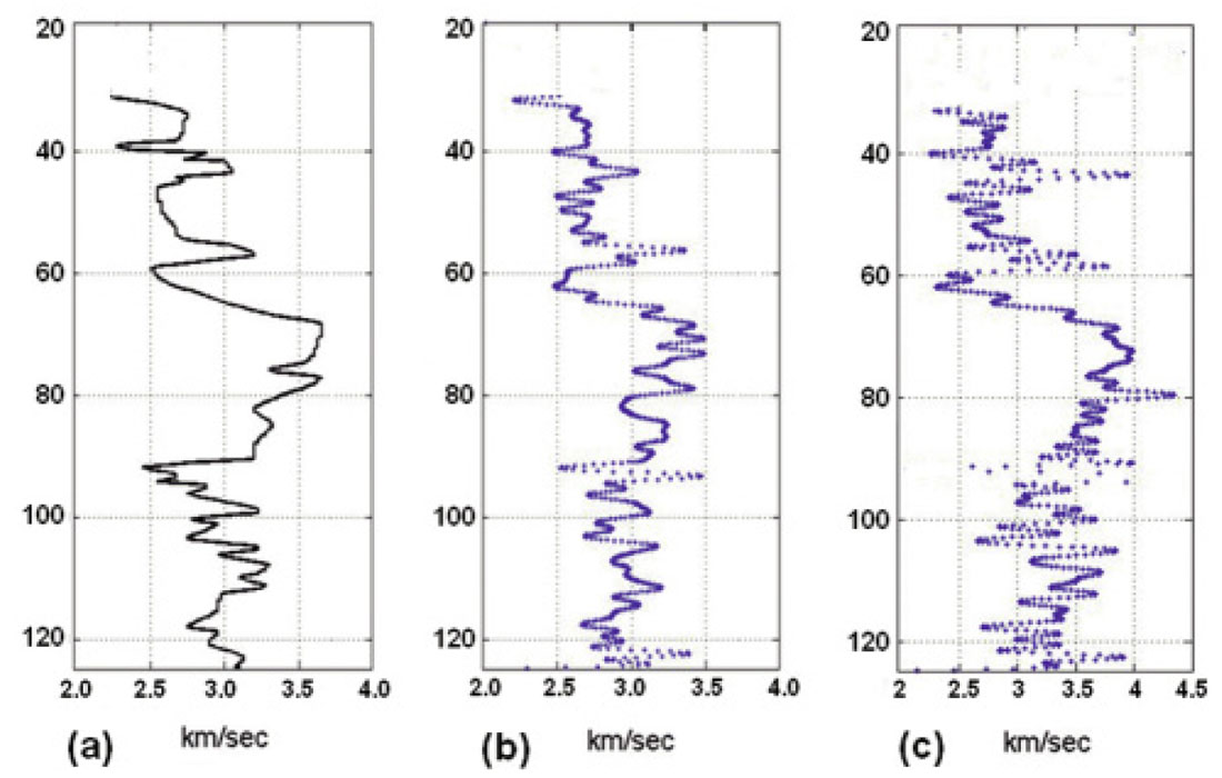
Even with noise-reduction on the raw field data, derived velocities will often appear wildly variable when plotted against depth. For example, on the velocity profile of Figure 13(a) we see many outlier values as well as rapidly varying jitter. Most outlier values can be eliminated by median filtering, and the velocity profile can be further smoothed by high-cut vertical wavenumber filtering. The effects of these smoothing operations are displayed on Figures 13(b) and 13(c).

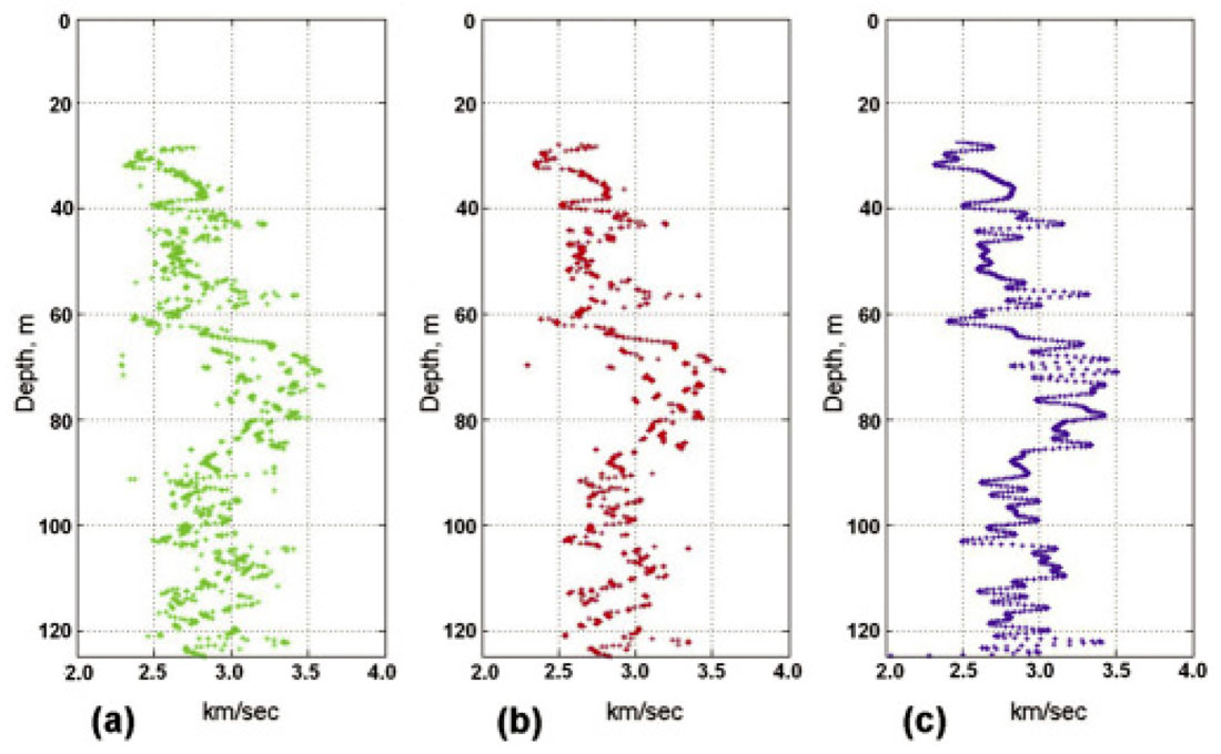
Figures 14(a) and 14(b) displays velocity profiles calculated using the refraction formula with manual and automatic firstarrival picks, respectively. Figure 14(c) shows a velocity profile obtained automatically using the time-shift method. With a water velocity of 1480 m/s, refraction analysis gave maximum velocity values of about 3600 m/s. These are about 10% lower than the maximum velocity values resulting from the timeshift calculation. On the time-shift-based velocity profile of Figure 14(c), spurious values occur at depths near 44 m, 58m, and 92 m. They are due to the fact that the first arrivals at these depths are particularly weak, reducing the effectiveness and accuracy of the phase alignment procedure.

Summary and Conclusions

The geophysical well logs presented in this study gave useful information regarding the near-surface geological and hydrogeological characteristics of the Paskapoo Formation at the Rothney Observatory site near Priddis, Alberta. Natural gamma-ray, resistivity, and neutron-neutron logs delineated the shale/sandstone bedding with good precision. Open-hole density and caliper logs clearly identified fracturing in the top 60 m of the well. A large fracture at 20 m depth and fractured thin sandstone beds (identified by the gamma log and density and caliper logs) appeared to be the source of fast-flowing groundwater that the driller estimated came from depths of 24 m to 28 m. Another large fracture, identified at a depth of 30 m by the density and caliper logs, acted as a groundwater sink in the uncased well. The temperature log indicated that, within a thick sandstone unit, there is a zone of warmer water inflow at approximately 85 m not identified by the driller. A driller-identified water-bearing zone, extending from 116 m to 122 m, did not have an obvious geophysical log signature. However, a perched aquifer in the vicinity would be consistent with the sharp sandstone-shale interface indicated at 116 m by the natural gamma-ray logs.

Full-waveform sonic (FWS) logs provided a large number of digital traces from which first-arrival times were picked after noise reduction. We used a minimum variance principle to develop automatic algorithms for finding time shifts that align first arrivals on windowed input traces. Averaging the shifted input traces reduced the deleterious effects of random noise on automatic picking routines. We formulated a first-arrival time-picking method that searches for the maximum of a modified energy ratio attribute calculated on noisereduced traces. Refraction analysis in a well bore was used to obtain estimates of P-wave formation velocities from the first-arrival times. However, simply dividing the intervals between receivers by the time shifts that resulted from alignment of multi-channel traces gave more accurate velocity values from the FWS data. Our implementation of these procedures in MATLAB code can be used to process thousands or tens of thousands of seismograms that make up a typical FWS log.

Acknowledgements

We thank the Alberta Ingenuity Centre for Water Research, NSERC, and the industrial sponsors of CREWES for their support of this study.