Deconvolution After Migration

Introduction

Deconvolution is a process that is normally applied before migration. However, deconvolution should also be performed after migration to enhance the resolution of the data. This concept has been practiced with some marine processing, but we have met considerable opposition when applying it to land data. We discuss some reasons why there is opposition to deconvolution after migration, present two reasons to deconvolve after migration, then present some examples. Deconvolution after a prestack migration is especially important.

Reasons to not migrate after deconvolution

Concern 1: Migration lowers the frequency content of dipping events

Migration lowers the frequency content of a dipping event to prevent aliasing, and a deconvolution may cause aliasing. That is true, however, if the project is in a sedimentary basin, the seismic data is reasonably flat, and a single trace deconvolution will be adequate to enhance the resolution of the data. If the data is structured, then a more elaborate deconvolution in the FK domain could be employed to accommodate dipping events in the FK domain. Some migrations are capable of deliberately migrating aliased events, and leave the events with higher amplitudes, and let the eye aid in interpolate the data.

Concern 2: Deconvolution will increase the noise

Not so. Deconvolution enhances the resolution and increases the amplitude of the wavelet by concentrating more energy in the peak. Deconvolution also tends to whiten or flatten the spectrum of the data where the signal to noise ratio (SNR) is greater than one. Energy outside this band should be attenuated with an appropriate band pass filter.

Concern 3: Deconvolution will produce artifacts

Some migration programs are created in sections that are cutand- pasted (stitched) together. A deconvolution after these types of migrations may reveal the stitching and be unacceptable. A deconvolution after migration may be more desirable to a client if this is the case.

Concern 4: A Kirchhoff migration already uses a whitening operator

A Kirchhoff migration should correlate the data with a diffraction that contains a wavelet. This correlation or matched filter would reduce the bandwidth of the data. (More on this later). However, most Kirchhoff migrations use a single valued diffraction to correlate with the data, and prevent this loss of resolution. It is then argued that there is no further reason to spectrally enhance the data.

Reasons to deconvole after migrate

We will present two reasons to deconvolve after migration and expect you to provide a third reason by trying “it”. The first argument is based on linear algebra and least-squaresmigration (LSM). The second reason will be based on a simple description of noise attenuation.

Migration is a transpose process

When modelling, the “forward process” spreads diffractions on the seismic sections with amplitudes that are proportional to the reflectivity. When migrating, the “reverse process” spreads energy along semi-circles, with amplitudes that are proportional to the seismic data. It can be shown that the transpose of a family of diffractions is a family of semicircles, implying that migration is a transpose process. This was pointed out by Claerbout in 1992 when he taught that many processes in exploration geophysics that we thought were inverse processes are really transpose processes. We will illustrate this with linear algebra.

Consider the forward process of modelling as

where D is a diffraction matrix, r a reflectivity structure, and s the modelled seismic section. A true inversion would be

providing D is invertable. It is usually not invertible so we make use of the least square method to get an estimate of the reflectivity from

(I will ignore a stability factor that will help invert the DTD matrix.) We become comfortable by assuming the DTD matrix is diagonally dominant, and approximate it with the identity matrix I, which has the convenient inverse that equals I, i.e.,

This allows us to write an alternate estimate for the reflectivity

where our “inversion” process has been approximated by a transpose process that we call migration.

What have we lost by dropping the D^TD part of the inversion? We contend that this is an essential part of our processing and will demonstrate this point by using least squares migration (LSM). But let’s back up and use more detail in out modelling process.

We conveniently left out any mention of a wavelet in the modelling. This is quite normal as in our modelling and migration we use single valued diffractions and semi-circles as it is more convenient, faster, and does a reasonable job. The wavelet was assumed to be part of the reflectivity structure.

Let us assume that we have a wavelet matrix W that can be multiplied with the diffraction matrix D to put wavelets on the diffractions, i.e.,

Now our reflectivity matrix r can really be a high frequency representation of the true reflectivity and we have the wavelet with the diffraction as it should be. The least squares solution is now

Removing the inversion part and going back to the transpose solution we get

This is quite interesting as we are now implying that we need to “convolve or correlate” the seismic data with another wavelet. That is multiplication in the frequency domain and that will narrow the bandwidth. That is correct, and if we did do that, we would end up with a zero-phase wavelet, typical of a true matched-filter. The peak of the wavelet would be higher and the noise attenuated. If we ignore the wavelet matrix, as in equation (5) then we do have a higher frequency migration with the same wavelet and more noise.

“But wait, there is more”.

We left out the inversion part again. Let me rewrite equation (7) again but in a form for some kind of dimensional analysis, i.e.,

In the central part, we have two wavelets in the numerator and two in the denominator. We end up on the right with our conventional migration D^Ts that still requires some inverse action with the wavelet W, i.e. deconvolution to recover the reflectivity. I am trying to show that a full inversion also applies an inversion (or deconvolution) of the seismic wavelet in s.

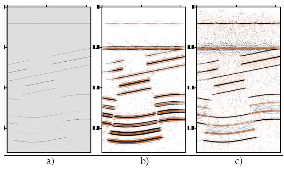
I illustrate with this concept with a true inversion that uses a full least squares migration (LSM). The full LSM is extremely computationally intensive and usually only simple models are shown. Figure 1 shows three panels with a reflectivity structure, a prestack migration from seismic data modelled on the structure, and a corresponding LSM. Notice the wavelet remains with the migration, but has been substantially removed in the LSM.

These results look and are impressive, but the modelling and inversion process did not contain noise, which enabled the high frequency content of the wavelet to accurately reconstruct the reflectivity. We contend that the same resolution in Figure 1c could have been achieved with a deconvolution to the migrated section in Figure 1b.

We are not negating the power of LSM as it has many useful applications, especially in its ability to recover missing data, and know it will be of great practical value in the future. At this point We are only using it to justify using deconvolution after migration. We point out that the “deconvolution” provided by LSM is most probably appropriate for dipping events where the resolution is defined normal to the dip, and not in a vertical trace.

Stacking and noise attenuation

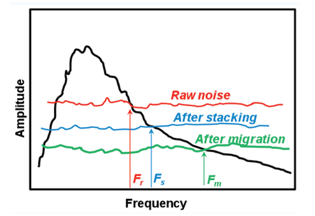
Deconvolution essentially tries to flatten the amplitude spectrum. However, when we flatten the spectrum, we flatten the signal and the noise. We generally consider the bandwidth of the signal, or reflection energy, to be the area on an amplitude spectrum where the signal is greater than the noise, i.e., SNR > 1. This is illustrated in Figure 2 which contains an exaggerated cartoon sketch of the amplitude spectrum of seismic data and three levels of noise. The first noise level represents the noise level in the raw data, the second is the reduced noise after stacking, and the third is the noise level after migration. Each time we reduce noise, we increase the bandwidth where the signal to noise ratio is greater than one, i.e., for the higher frequencies from Fr to Fs and then Fm. There is also a corresponding reduction of the lower frequencies. A deconvolution at each noise level will tend to flatten the signal spectrum and a bandpass filter will remove the noise where the SNR < 1.

Migration should reduce noise and increases the high frequency content of the data that is above a SNR of one. I use the word should, because some migrations retain noise:

1. deliberately for appearance purposes,
2. the algorithm can’t remove the noise, or
3. because an antialiasing filter was not used.

In these cases a deconvolution after migration may not improve the result.

Dips on a seismic section (before migration) are limited to less than 45 degrees. Dipping energy above 45 degrees is noise, and should be removed by the migration algorithm. This is done by the antialiasing filter in a Kirchhoff migration, and a natural part of the frequency domain algorithms. However some algorithms, such as finite difference, cannot remove this noise and it may be spread over the entire section. In these latter cases, a dip filter should be applied to the seismic data to remove noise above dips of 45 degrees.

Earlier in our careers we had to add noise back to a migrated section to make it look “more interpretable”. To some a migrated section with complete noise attenuation may look “wormy”. A deconvolution tends to remove this “worminess”.

An example of deconvolution after migration

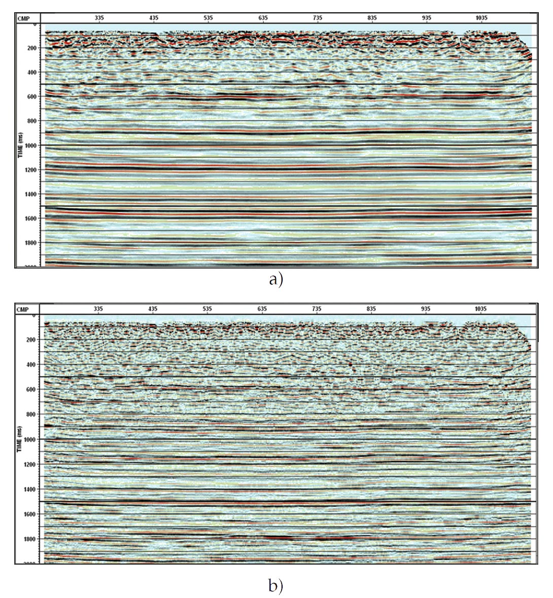
The CREWES project acquired data on a short 2D line, in the area of Hussar, Alberta Canada, for evaluating low frequencies. A noisy 2D seismic line was chosen that used a low-dwell sweep from 1 to 100 Hz, into the vertical component of a 3C 10 Hz phone. The data was processed to a flat datum at the central elevation. Deconvolution, gain recovery, and statics were applied to the data prestack data. The data was then prestack time migrated using the Equivalent Offset method (EOM). The migrated section is shown in Figure 3a and the migration followed by a spiking deconvolution is shown in Figure 3b. The increase in resolution with deconvolution after migration is evident.

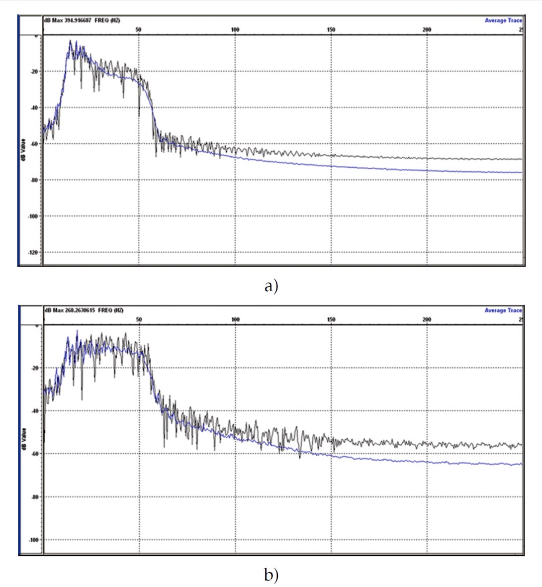
The amplitude spectra of the Hussar data are compared in Figure 4, with (a) the prestack migration, and (b) after deconvolution. Note the flatter amplitudes of the deconvolved section in the energy band of the seismic data that was constrained by a filter.

Comments and Conclusions

Figure 2 illustrated the increase in bandwidth after stacking and migration. Stacked data is normally deconvolved before a poststack migration. This deconvolution is not available to a prestack migration, and may therefore have a lower bandwidth than a corresponding poststack migration. In this case, deconvolution after a prestack migration is essential.

There may be a need to develop a 2D deconvolution that is applied after a prestack migration for highly structured data.

The ability of deconvolution after migration may have a significant impact on full waveform inversion (FWI) by providing much lower frequencies in the seismic data.

We recommend using a prestack migration with competent noise attenuation. An example would be a Kirchhoff migration with a good antialiasing filter, or filter dips greater than 45 degrees. Then try a simple spiking deconvolution to evaluate any improvement. If you see an improvement, use a more appropriate time varying algorithm such as a Gabor deconvolution (Margrave et al. 2011) to maximize the resolution at all parts of the section.

Acknowledgements

We thank all CREWES sponsors, staff and students for their support.