Comparison between faults extracted from seismic and Elastic Dislocation Modelling

Introduction

Most fault enhancement techniques rely on enhancing the discontinuities within the seismic signal. However, there is a large variety of phenomena that cause discontinuities in the seismic signal. Furthermore, fault heaves are lower than the Fresnel zone width thus not fully resolvable and as a result, faults are often poorly imaged and can be blurry and discontinuous. In order to overcome some of the inherent limitations of fault enhancement of small scale faults, we use Elastic Dislocation (ED) modelling to provide an independent means of assessing sub-seismic fault geometry and distribution.

ED modelling assumes that the main control on small fractures and small scale fault distribution and density is the coseismic strain perturbations that occur around large (seismically visible) faults (Dee et al., 2007). From the displacement on the large faults, and knowledge of the external stress field and rock properties, the stress distributions and thus failure characteristics can be calculated, by modelling elastic dislocations in the wall rocks enveloping a fault whose displacement distribution is known (e.g. from seismic mapping) (Dee et al., 2007). ED modelling ultimately predicts the orientation, distribution and mode (e.g. pure tensile vs. shear and hybrid fractures) of secondary fault/fractures.

Using a case study from Tunisia, we compared the small scale fault distributions predicted in the fault enhanced volume with those predicted by the ED method. Faults that can be cross validated using these two methods can be more confidently interpreted.

Seismic fault enhancement techniques – methods and limits

The majority of the seismic fault enhancement technologies measure the discontinuities of the seismic signal. But those discontinuities can have many sources:

• Genuine faults
• Noise (coherent and noncoherent)
• Acquisition footprint (can sometimes be observed on fault cubes as large vertical features following acquisition direction)
• Processing artifact (migration wing interfering with genuine signal, multiple interference, etc.)
• Dipping event (for instance the Variance/Coherence volumes use a vertical window, which enhances dipping beds)
• Non-stratified objects (edge of salt diapir, any intrusion/ diapir, etc.)

The noise can be reduced through reprocessing, filtering and smoothing. However there is always the risk of losing small genuine faults. Therefore, enhancing faults is always a compromise between quality of extraction and size of the objects.

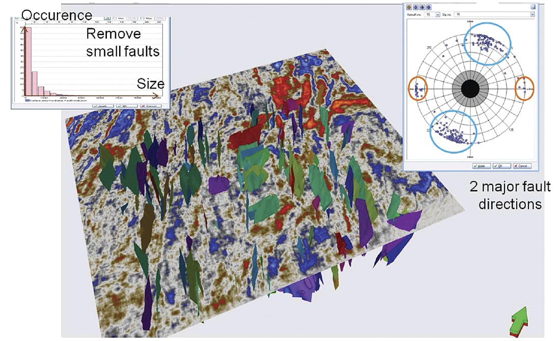
The acquisition footprint can be reduced using directional filtering. This can be done within the Ant Tracking workflow (Pedersen et al., 2003). The filtering can be done before or after the extraction of fault patches and also enables the user to analyze different fault sets (Figure 1).

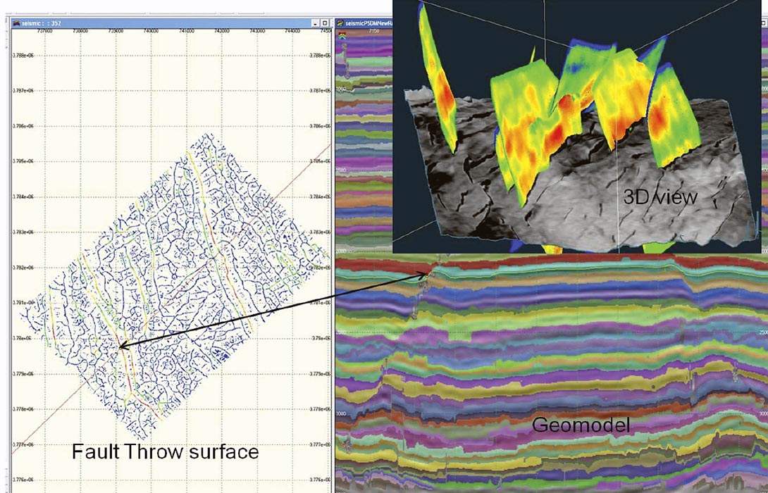
The vertical estimation can be used to differentiate genuine faults from processing and acquisition artifacts. This can be done using the PaleoScan workflow (Figure 2) as describe by Bates (Bates et al., 2009). Of course reprocessing is always recommended when possible to remove any artifacts.

The effect of dipping events can be mitigated by a dip steering approach (de Groot and Bril, 2005). A non stratified event can be more difficult to detect, however, such events are unlikely to have a consistent displacement. Therefore, the displacement calculation should help to identify such features. There are a large variety of methods, which help to separate genuine faults from other discontinuities, however, it is often at the cost of reducing genuine signal.

Elastic dislocation modelling

This method assumes that the strain distributions around large scale faults are primarily controlled by the slip on the large faults (Dee et al., 2007). ED theory is a proven method for predicting the distribution of co-seismic deformation (Bourne and Willemse, 2001; Healy et al., 2004). For example, (Healy et al., 2004) accurately modelled the secondary faulting that formed after the 1980 El Asnam earthquake. For a more complete review of ED theory see (Dee, et al. 2007). We use FaultED, a Badley Geoscience software package, to perform the Elastic Dislocation model. FaultED is a boundary element - elastic dislocation program for determining the strains and structures associated with seismically mappable faults (Dee, et al. 2007).

Details of required inputs:

Fault surfaces with fault polygons

A detailed, well built structural model will produce the most reliable outputs, as the model will inherently produce results that look realistic. Therefore, all major faults in the study area need to be included.

Regional stress magnitude and direction

This is a critical factor to get right as it can either enhance a trend or completely overprint it if applied incorrectly. To determine an accurate regional stress value it is necessary to know the geological history of the study area and the nature and timing of slip on the faults. An important point to remember is that the regional stress parameters at the time of deformation are required, not the present day stress parameters. If an area has been reactivated in different orientations then the results could be misleading. In general, if the faults are purely dip slip, then the maximum extension direction is typically perpendicular to the main fault trend.

Geomechanics

This parameter, along with the background stress, enables FaultED to compute strain tensors, which are calculated from the major faults, from stress tensors and hence calculate the total stress field and any associated fracturing (Dee et al., 2007). To do this correctly, information on rock strength (e.g. friction coefficient, ultimate strength, cohesive strength, Poisson’s ratio) is required. However, in most cases published estimates for “typical” rock properties are utilised as the required tests are not typically preformed in the hydrocarbon industry. FaultED does not incorporate variations in mechanical stratigraphy but assumes linear elasticity.

Case Study: Tunisia horst terrace

We have applied a fault enhancement workflow based on the Ant Tracking algorithm and the elastic dislocation modelling to a Tunisian dataset. The area of interest is a terrace on the side of a main horst. This area is about to be developed. Prior to drilling development wells, it is crucial to understand the inner structure of the terrace. It will help prevent drilling hazards, understand potential compartmentalisation and determine an optimum production strategy.

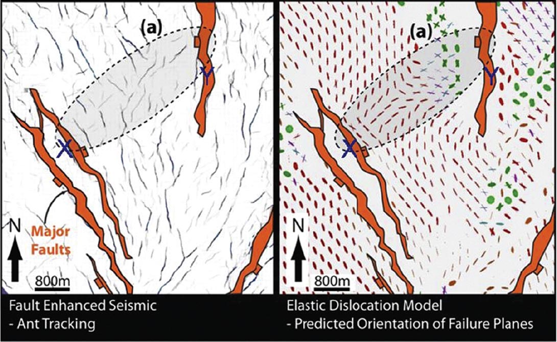
The terrace is bounded by four major faults (Figure 3) that are used as input in the elastic dislocation modelling. In the fault enhancement volume, we observe an unusual trend (SW – NE) between the two major bounding faults (Figure 3a). This fault trend is also observed in the elastic dislocation model. The two methods were performed independently and rely on different hypotheses. Therefore, we have gained confidence that the SW – NE fault trend is genuine and should be used in future geological and reservoir models.

Conclusions

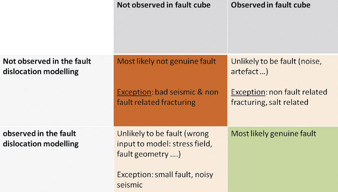
Combining fault enhancement techniques and elastic dislocation modelling is a robust way to identify fault features at the edge of the seismic resolution. It also helps to isolate discontinuities that are not genuine faults. In Figure 4, we describe the different outcome we might obtain, when the two methods are combined.