Summary
A research project was undertaken in August 2011 for continuous passive monitoring of a multistage hydraulic fracture stimulation of a Montney gas reservoir near Dawson Creek, B.C., with the main objective of investigating low-frequency characteristics of microseismic events. This work was motivated by a recently discovered class of long-period longduration (LPLD) events, interpreted to represent slow slip along pre-existing fractures. The field deployment included a 6-level downhole toolstring with low-frequency (4.5 Hz) geophones and a set of 21 portable broadband seismograph systems. Time-frequency analysis of extracted high- and lowfrequency microseismic events made use of the short-time Fourier transform. Observed low-frequency microseismic signals included tremor phenomena at various time scales, from a few seconds to the entire duration of high-pressure fluid injection, in addition to inferred regional earthquakes located ~150 km from the monitoring site. Relative to previously documented LPLD events from the Barnett, differences in low-frequency response for this Montney stimulation are interpreted to reflect a lower degree of complexity of preexisting and induced fracture networks. Analysis of lowfrequency microseismic signals shows promise for improving geomechanical understanding of fracture processes.
Introduction
In recent years, seismologists have increasingly recognized the significance of low-frequency earthquakes. Terms such as non-volcanic tremor and slow-slip earthquakes are often applied to describe this phenomenon, which constitutes a significant component of the spectrum of energy radiated from earthquake fault systems (Beroza and Ide, 2011). Das and Zoback (2011) recently documented a new class of fracinduced microseismicity, long-period long-duration (LPLD) events, that have similar characteristics to some classes of low-frequency seismic activity. LPLD events are distinguished from conventional high-frequency microseismic events by their relatively low frequencies (10-80 Hz), long durations of 20-50 s, and some waveform characteristics similar to tectonic tremor in fault systems. By analogy with tremor-like phenomena observed in a variety of fault systems (e.g. Shelly et al., 2007), Das and Zoback (2011) interpreted these signals as slow slip activated on pre-existing fracture systems by the hydraulic fracture treatment.
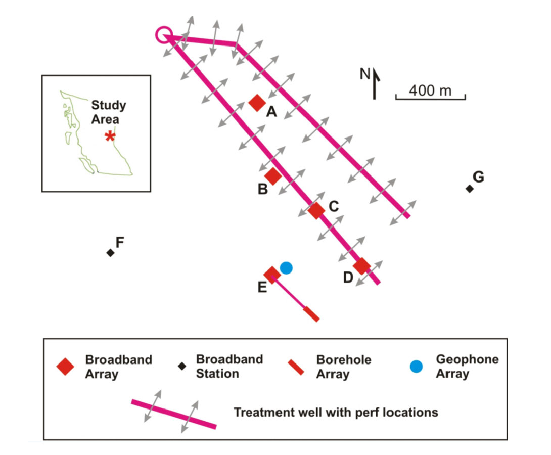
With these considerations in mind, a research project to acquire microseismic data was undertaken August 7-29, 2011 near Dawson Creek, B.C. Named the Rolla Microseismic Experiment (RME), this work involved recording of several multistage hydraulic fracture treatment programs performed in two horizontal wells (Figure 1). The microseismic data were collected using both surface and borehole sensors. The borehole toolstring consisted of a 6-level low-frequency system with downhole digitization. Surface sensors included a 12-channel array with a mix of vertical-component and 3-C geophones, and 22 broadband sensors (Trillium Compact seismometers and Taurus digitizers) deployed in 7 localized arrays over an area of ~ 0.5 km2. Data acquisition parameters are summarized in Table 1.
The unusual setup was employed to investigate multiple objectives. First, microseismic monitoring was performed using both surface and borehole equipment to compare both acquisition strategies in order to determine their mutual advantages and inconveniences such as ease of deployment, costs, detectability of events, other signals and associated noise levels. The experiment was also unusual in that both broadband and short-period equipment was deployed. The approximate lowest recording frequencies for the various sensors are: broadband surface-based seismometers, 0.0083 Hz (= 120 s); borehole equipment, 0.1 Hz; short-period surface array, 5 Hz. Data analysis of the variously recorded signals thus helps to reveal if significant energy is present below the low-frequency limit (~ 10 Hz) imposed by most standard monitoring equipment. It also may obscure proper identification of so-called slow earthquakes (Ide et al., 2007) occurring on much longer time scales than conventional earthquakes resulting from abrupt brittle failure.
| Manufacturer | Type of Sensor | Number of Sensors | Sample Rate (ms) | Start/End Dates | Sensor Spacing |
|---|---|---|---|---|---|
| Table 1: Summary of data-acquisition parameters. | |||||
| Spectraseis | 4.5 Hz 3C geophones | 6 | 0.5 | Aug. 15-18 and Aug. 21-25 | 32 m borehole |
| Nanometrics | Broadband seismometer (Trillium Compact) | 21 | 2.0 | ~ Aug. 8 to Aug. 27 | 50 m (4-element surface array) |
| ESG | 10 Hz geophones (mix of Z and 3C)1 | 8 | 0.5 | Aug. 15-18 | 20 m (8-element surface array) |
| 1Data from the surface geophone array are not used in this paper. | |||||
In this paper, we first describe the geological setting and operational setup for the RME. Next we outline the results from conventional microseismic analysis of the downhole observations, which focus on high-frequency microseismic events. We then undertake time-frequency analysis of the continuous datastream using short-time Fourier transforms to examine variations in local frequency content and highlight slow-deformation processes. This approach is motivated by similar analysis of acoustic emissions generated during laboratory rock-fracturing experiments, which have greatly aided in improving our understanding of active microcracking and deformation processes (Benson et al., 2008; Thompson et al., 2009).
Geological Setting and Operational Setup
Significant gas reserves are hosted by the Triassic Montney Formation in northeastern British Columbia and northwestern Alberta. Although estimates of natural gas in place are highly variable, ranging from 80 to 700 Tcf, in recent years production has increased dramatically to over 400MMcf/d (Walsh et al., 2006). The Montney Formation is an extensive siliciclastic-dominant unit that occurs from west-central Alberta to northeast British Columbia (Dixon, 2000); in the area of this study, it is overlain by the Triassic Doig Formation and underlain by the Permian Belloy Formation. The depositional environment of the Montney ranges from shallow-water shoreface sands to offshore marine muds (NEB, 2009). The reservoir rocks consist of interbedded shale, siltstone and sandstone layers, dominated by shale and silty shale (Dixon, 2000). Thickness can range up to 300m, while porosity is very low, ranging from 1.0-6.0% (NEB, 2009).
The overall layout of field equipment and relative location of the two treatment wells (A and B) are shown in Figure 1. The 10-stage fracture treatment program in well A took place August 15-18 and the 11-stage treatment program in well B took place August 21-25. Layout of the field equipment commenced August 8, and continuous recordings using surface sensors commenced prior to the start of the first stage of hydraulic fracturing. The broadband seismograph units recorded data continuously until August 27, whereas the surface geophone array was decommissioned on August 18 and thus only recorded the 10-stage frac treatment in well A.
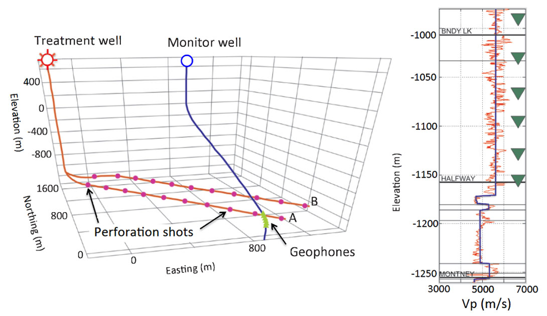
The six borehole array sondes were deployed on production tubing in the deviated monitor well (Figure 2). The geophone sondes were located a few hundred m above the reservoir unit, and coupling of the sondes to the wellbore casing was achieved by setting the tubing down on a packer. The total vertical aperture of the array was 160m. The array was retrieved and the data downloaded between the hydraulic fracture treatment programs in wells A and B, and again after completion of the well B treatment.
Analysis of high-frequency signals
Data recorded using the downhole arrays were processed using a workflow that included:
- Instrument response correction to convert raw amplitudes to units of m/s;
- Analysis of perforation shots to calibrate the background velocity model and determine sonde orientations for the two deployments;
- Automatic event detection using an amplitude-based triggering algorithm;
- Rotation of recorded signals from original orientations (axial plus two mutually perpendicular components in the plane locally perpendicular to the borehole) to fixed orientations (vertical, east-west, north-south);
- Interactive picking of P- and S-arrivals plus event classification;
- Determination of hypocentre locations using a least-squares algorithm;
- Estimation of event magnitudes based on the Brune model.
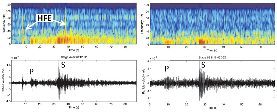
Examples of waveforms recorded from perforation shots together with time-frequency analyses are shown in Figure 3. As expected due to the volumetric nature of explosive sources, the waveforms are dominated by the direct P-wave. It is also possible to discern S-wave arrivals, which is important for calibration of the velocity model. For the closest shot location (~350m), the data contain usable signal up to the Nyquist frequency (1 kHz). The high-frequency content diminishes with distance due to the effects of anelastic attenuation. Waveform examples of high-frequency microseismic events are presented in Figure 4. In this case, the S-wave arrival has the highest amplitudes. The frequency content of these signals is predominantly concentrated above 100 Hz, and the bandwidth decreases with distance due to the effects of attenuation.
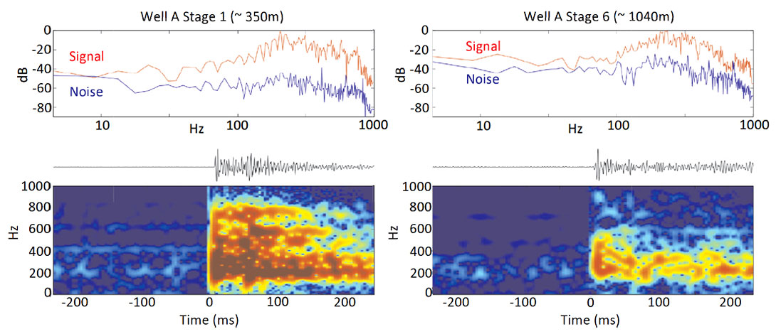
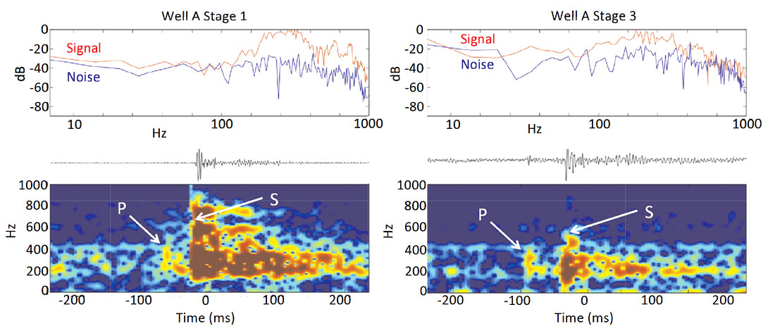
Figure 5 shows the computed moment magnitude (Mw) for all detected events, plotted versus distance from the centroid of the downhole geophone array. Graphs such as these are useful QC tools to identify magnitude anomalies and to assess the magnitude detection threshold. The detection threshold is a function of distance and refers here to the magnitude above which detection probability is approximately 100%. It is obtained by solving

where ω = 2πf is angular frequency, R = 0.63 is the average radiation pattern for S waves (Boore and Boatwright, 1984), ρ is density, r is source-receiver distance in m, VS is shear-wave velocity in m/s, QS is the shear-wave quality factor, and Amax is the maximum level of background noise in m/s. Here, detection limit refers to the magnitude below which detection probability is reduced to zero; the formula is similar to equation (1), except that Amax is replaced with Amix the minimum level of background noise. The parameters used here to evaluate detection threshold/limit are: f = 200 Hz, VS = 2500 m/s, ρ = 2500 kg/m3, QS = 5000, Amax = 6.5 10-9 m/s, Amax = 3.25 10-9 m/s.
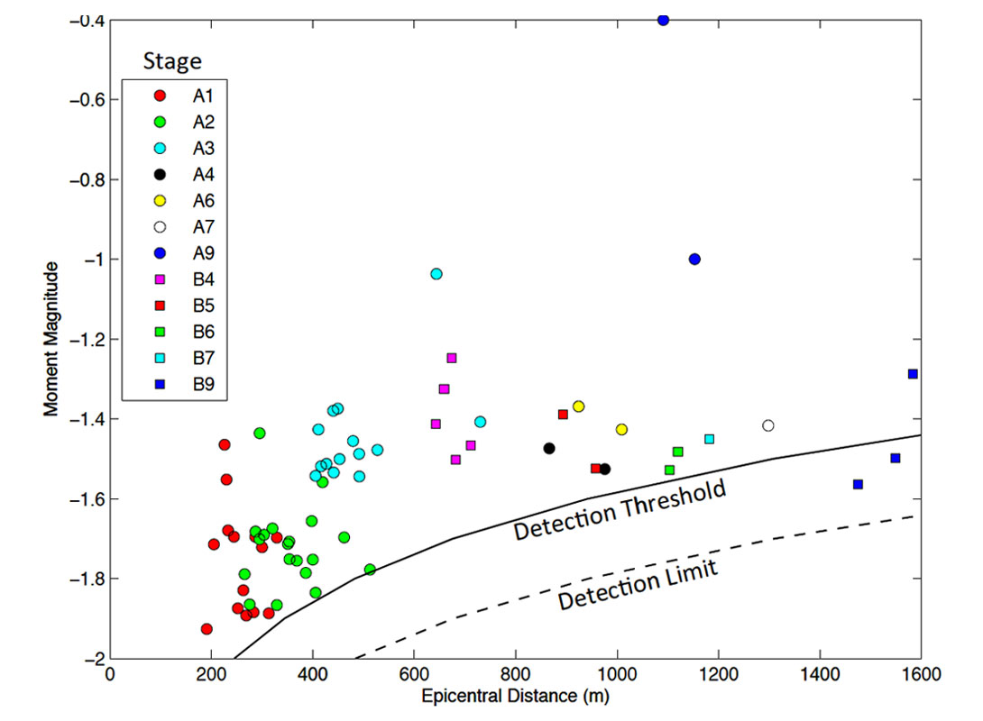
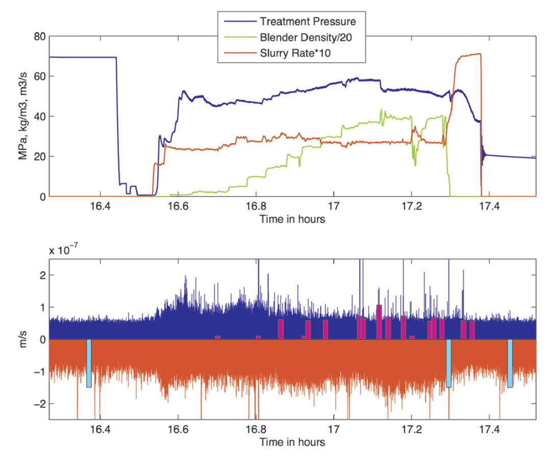
Figure 6 shows a synoptic plot comparing recorded microseismic data over the duration of a treatment stage with pumping curves (downhole treatment pressure, blender density and slurry rate). The time series in this figure is constructed by combining positive values from high-pass filtered data ($>200 Hz) with negative values from a low-pass filtered trace ($< 50 Hz). The purpose of this is to highlight simultaneously both high-frequency and lowfrequency responses. Also shown are detected high-frequency events (indicated by positive bars) and tube waves (indicated by negative bars). Some salient features of this plot are:Amplitude modulation of both high- and low-frequency microseismic data, evidenced by the envelope of the amplitude values, shows a trend that appears to correlate with the treatment pressure curve. For most other treatment stages, this amplitude modulation is more apparent for the lowfrequency data. As discussed below, this phenomenon is interpreted as tremor associated with pumping noise generated at the treatment wellhead.
- Potential high-frequency events are marked by high-amplitude spikes in the high-pass filtered microseismic time series. Locatable events, where both P and S-wave arrivals are visible as shown in Figure 4, do not occur until the second half of the treatment stage with proppant levels are increased as indicated by the blender density (green curve in Figure 6).
- Low-frequency events (LFE’s) are marked by high-amplitude spikes in the low-pass filtered microseismic time series. In some cases these correlate with high-frequency events, and in other cases these correlate with tube-wave arrivals.
Analysis of low-frequency signals
A systematic search for low-frequency signals was carried out using an approach similar to steps 1, 3 and 4 in the highfrequency workflow. In this case, however, two low-pass filters were first applied to the data, with cutoff frequencies of 100 Hz and 25 Hz, respectively. All events that were detected with the 25 Hz cutoff but not with the 100 Hz cutoff were examined using a time-frequency analysis approach based on the short-time Fourier transform. This dual-detection approach was used to eliminate unnecessary analysis of high-frequency events that also contain significant signal content below 25 Hz. Due to the long duration of LPLD events, an initial long time window (~ 5 minutes) was used. The time window was then reduced, on a case-by-case basis. A total of 50 events were identified in this way, of which 24 are of long duration (> 20s) and the remaining are of shorter duration. The former is referred to here as longduration low-frequency tremor, and the latter are referred to here as low-frequency events (LFE’s). In addition, the envelope of the low-frequency signals (Figure 6) was investigated. Each of these types of low-frequency signals is considered separately in the following sections.
Figure 7 shows an example of a long-duration low-frequency tremor signal. Although this has some characteristics of LPLD events as described by Das and Zoback (2011), the frequency content is significantly lower (< 20 Hz). Figure 8 shows two examples of low-frequency events (LFE’s) followed by subsequent high-frequency events. This apparent causal relationship between these classes of microseismic activity occurs in about 20% of the cases examined.
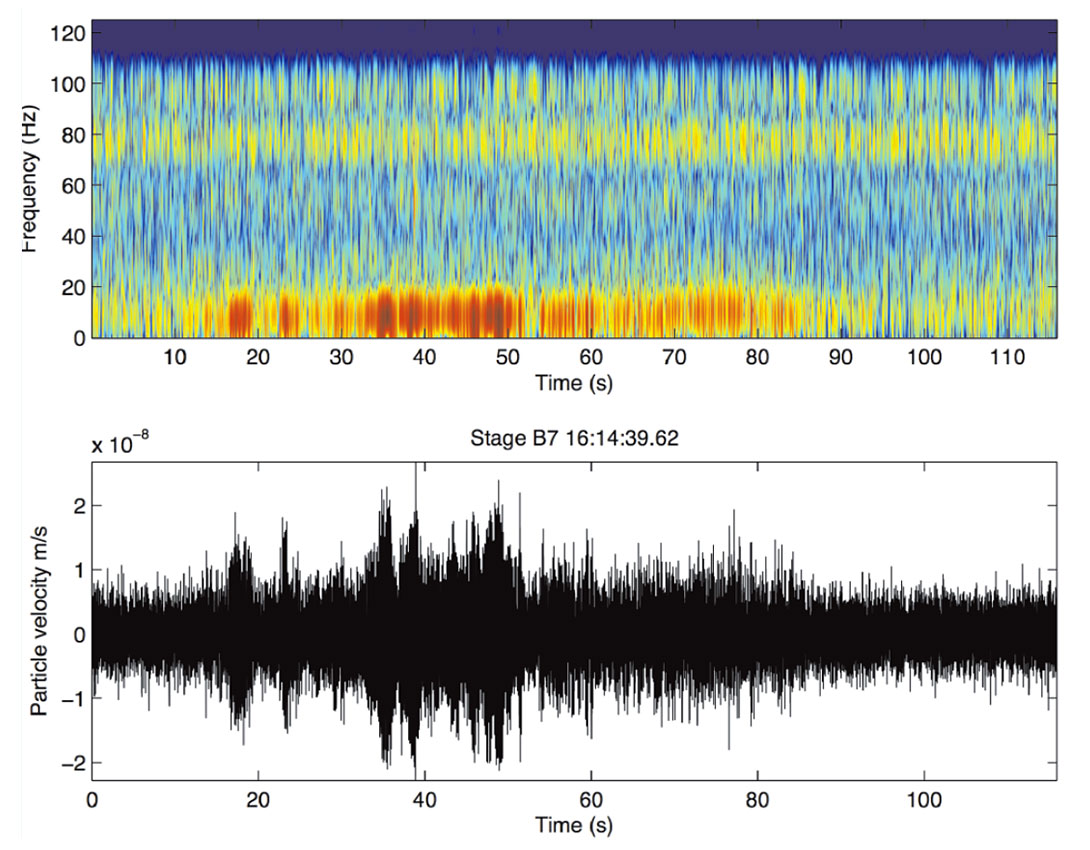
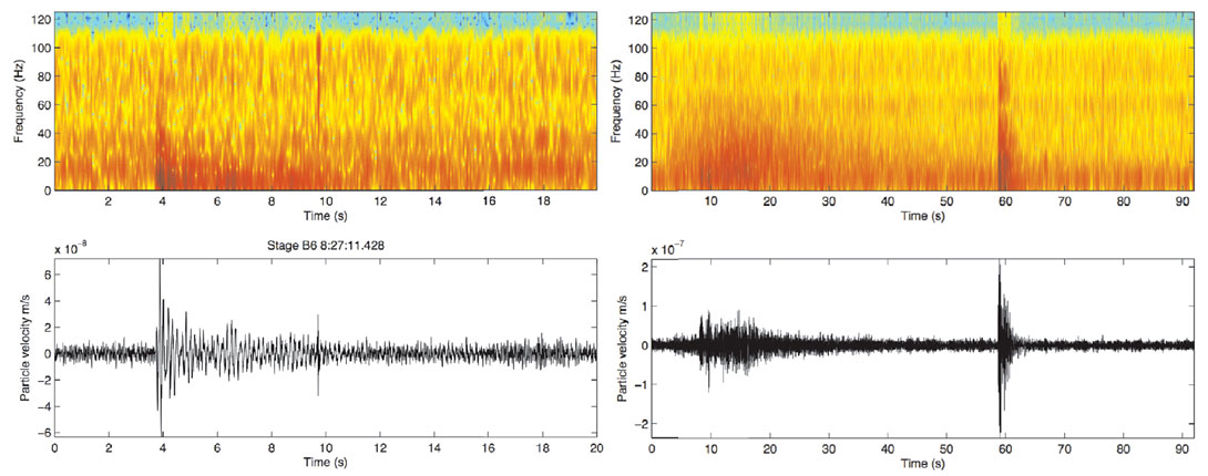
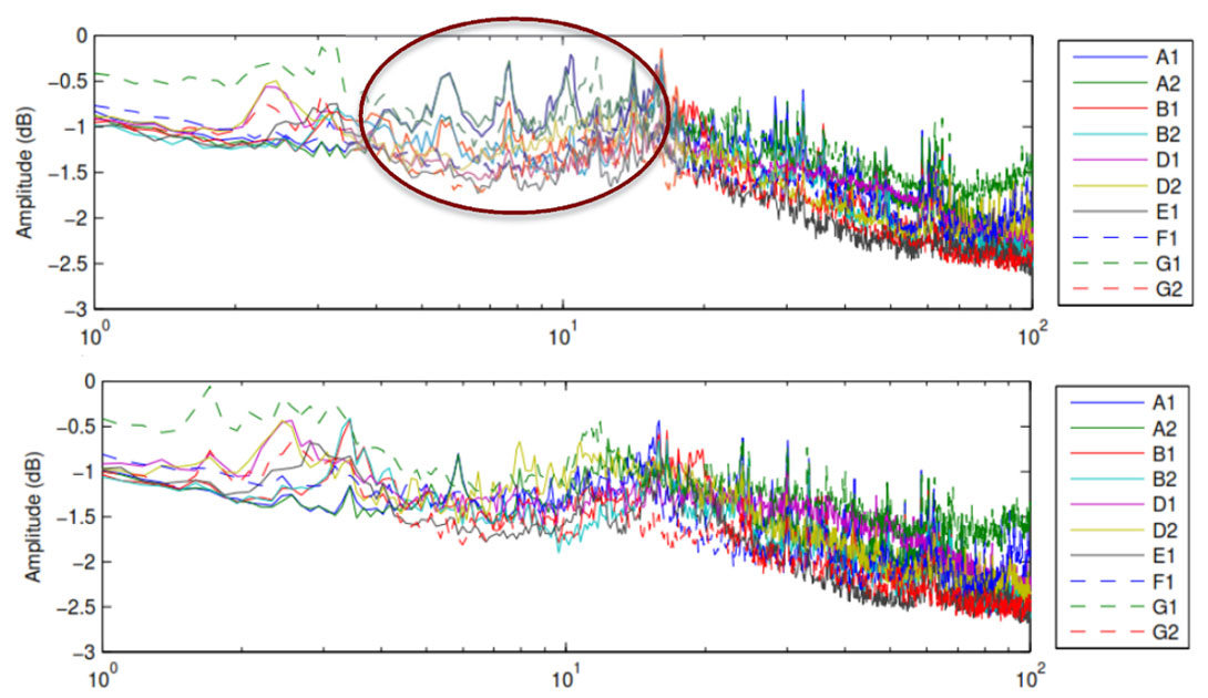
Figure 9 shows an analysis of the average spectral content of vertical-component signals recorded on surface broadband seismograph stations (Figure 1) during and before the stage 3 hydraulic treatment in well A. The data recorded during the treatment contains spectral peaks centred at 5.5, 7.8 and 11.0 Hz, respectively. Although the spectral peak at 5.5 Hz may be related to background noise, the others are absent or significantly reduced for the non-frac time window, which is assumed to characterize the background noise levels. These peaks are most conspicuous for array A (located closest to the treatment well pad), less conspicuous for array B (located about 400 m south of array A), and virtually absent for the other arrays. This pattern suggests that the source of the spectral energy in this low-frequency band comprises pumping equipment associated with the hydraulic fracture stimulation.
In order to examine low-frequency tremor extending over the duration of the fracture treatment, we computed an amplitude envelope function for the continuous microseismic data using the following approach:
- A low-pass filter was applied, with a cutoff frequency of 25 Hz.
- The absolute value of the data was computed.
- A 5-s running median filter was applied to the rectified data to remove amplitude spikes.
Figure 10 shows the low-frequency tremor envelope computed in this fashion for treatment stages 1-8 of well A. Stages 9 and 10 are note considered here, as the data contain strong signals from teleseismic earthquakes that distort the calculations. To facilitate comparison, the envelope signals are aligned based on the start time of each stage. While details vary from stage-to-stage, this plot indicates that, for this low frequency band, long-duration tremor signals are characterized by similar amplitude levels for each stage. Since the distance from the monitor well increases from stage 1 to 8, this analysis suggests that (to first order) the signal does not vary with distance from the treatment location.
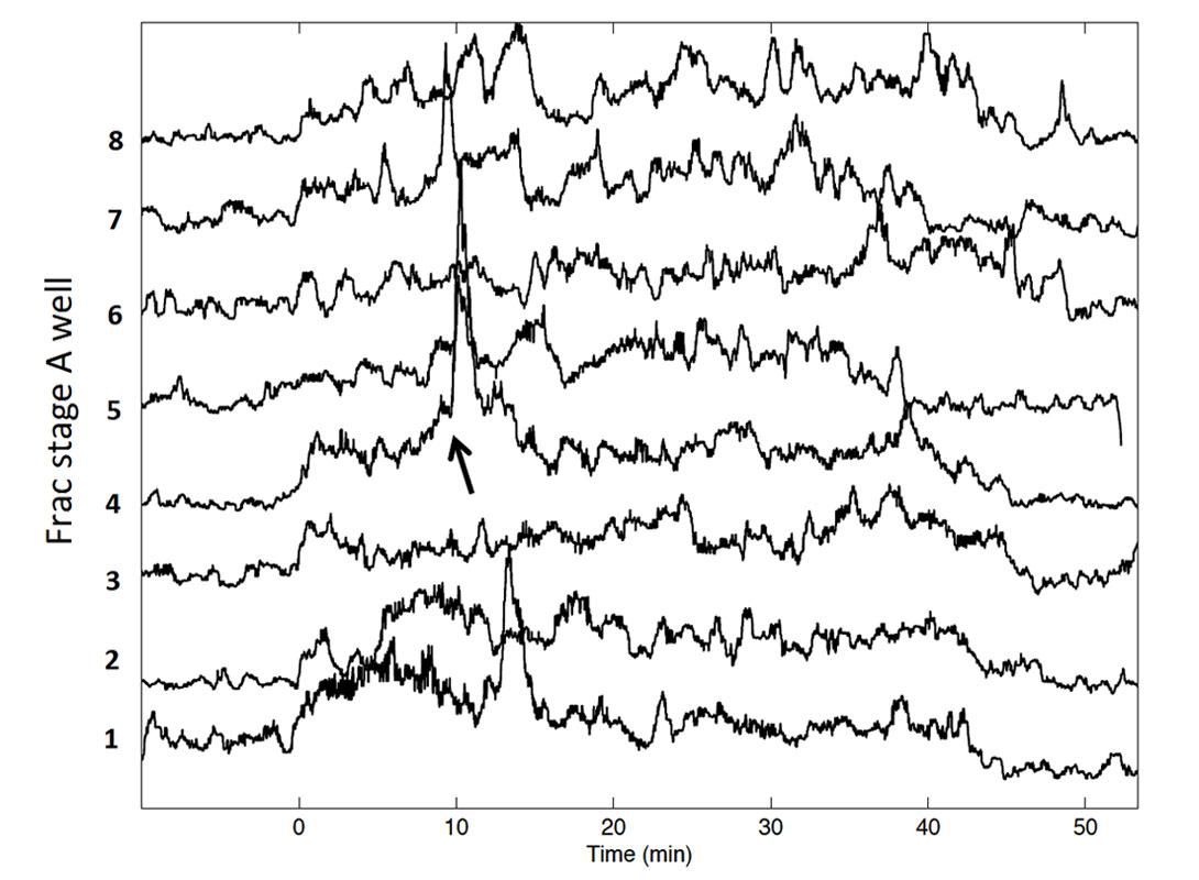
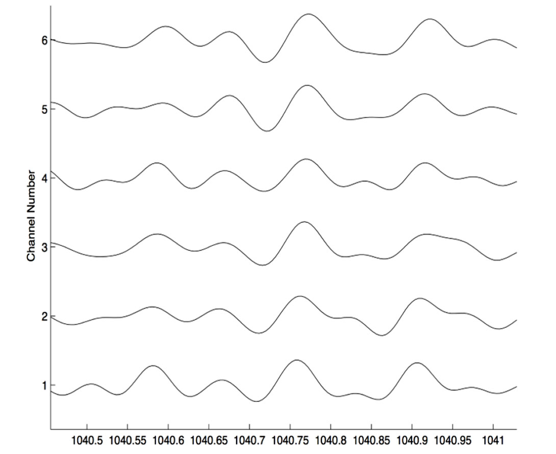
Figure 11 shows an enlargement of a representative short time window containing low-frequency tremor signals. The signals occur predominantly on the vertical component, suggesting a dominantly vertical polarization direction. In addition, the apparent velocity of the signals is > 10 km/s. Taken together, these characteristics suggest that the tremor signals are comprised largely of near horizontally propagating S-waves.
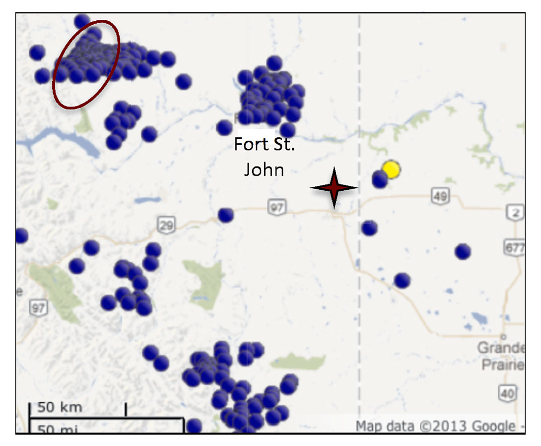
It is important to distinguish between potential LPLD events associated to the hydraulic fracturing treatment and local earthquakes. For example, Fig 12 shows a number of recorded signals that are interpreted here as regional earthquakes that are unrelated to this hydraulic fracture treatment. When viewed using suitably long time windows, several of these events exhibit pairs of arrivals that are dominated by frequencies less than 20 Hz and separated by ~ 18s. If these represent direct P and S arrivals from an earthquake, this implies an epicentral distance of about 150 km, based on the velocity model used by the Alberta Geological Survey to determine earthquake locations (Virginia Stern, pers. comm., 2013):
| Depth | P | S |
|---|---|---|
| 0-36 | 6.2 km/s | 3.57 km/s |
| 36 | 8.2 km/s | 4.7 km/s |
Assuming that this is an earthquake, Figure 12 shows a circle identifying possible locations of the epicenter. This circle encloses an earthquake-prone area west of Fort St. John. The event is thus interpreted as a natural seismic event, unrelated to this hydraulic fracture treatment, located about 150 km from the monitor well. No events from this region are listed during August 2011 in the GSC’s online national earthquake catalog (http://www.earthquakescanada. nrcan.gc.ca/stndon/NEDB-BNDS/bull-eng.php, accessed on 2013/02/01), suggesting that its magnitude is less than the detection threshold of M ~ 2.5 for the catalog.
Discussion
Based on our experience from western Canada, high-frequency microseismic events from this hydraulic-fracture stimulation program are sparse relative to other regions. In particular, it is not unusual to record > 100 events per treatment stage for the rate/volume/pressure parameters used here. Although the paucity of events may, in part, reflect the relatively large lateral separation of the monitor well from the treatment zones for this experiment (350-2000 m), we remark that perforation shots were well recorded to a distance of 2000m. Instead, we interpret much of the reduced high-frequency signals to a less brittle response to high-pressure fluid injection of the silty shale Montney reservoir unit in this region than for other unconventional reservoirs in western Canada.
Another noteworthy attribute of the high-frequency microseismicity is an apparent delayed onset of locatable events (i.e., events that contain clear P and S arrivals) until the proppant concentration, represented in Figure 6 by the blender density, achieves ~30% of its maximum value. Prior to this point in the treatment, deformation associated with tensile opening of the hydraulic fracture appears to produce fewer and weaker microseismic events. Under the prevailing geomechanical conditions for this treatment, this behavior may reflect a period of less brittle deformation that occurs before injection of proppant into the reservoir.
Although only 50 low-frequency events were detected during the stimulation programs, the signals documented here provide potential insights into fracturing processes. In particular, we interpret the low-frequency signals (tremor) to mark deformation processes that are otherwise aseismic. In addition, the precursory temporal relationship observed in some cases (Figure 8) suggests a possible causal relationship sometimes exists between tremor and subsequent high-frequency deformation processes.
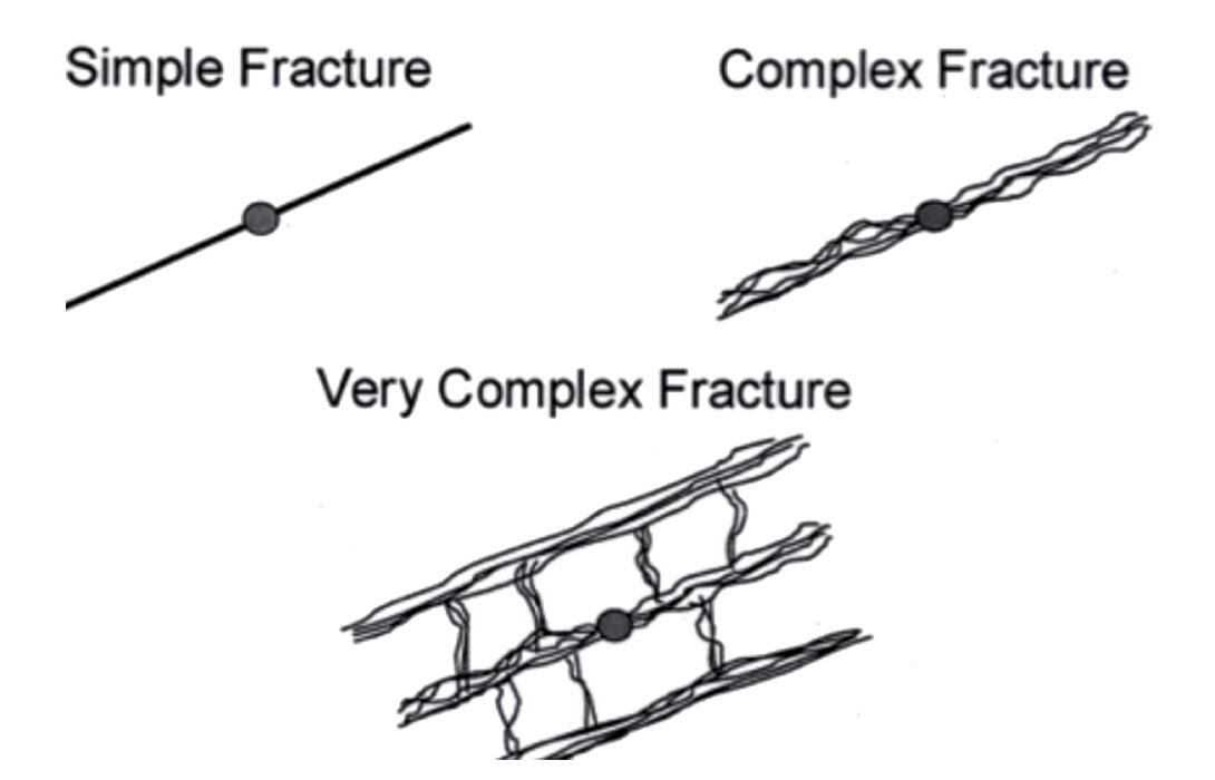
It is also noteworthy that none of the low-frequency signals observed here strongly resemble LPLD events from the Barnett shale, which have frequencies of 5-50 Hz and durations of 30-50 s (Das and Zoback, 2011). In their interpretation, Das and Zoback (2011) suggested that LPLD events could represent slow slip on fracture zones near the treatment well. They also suggested that the abundance of LPLD events depends on the density of fractures in the treatment zone. The Barnett shale is noted for fracture- network complexity (Fig. 13; Maxwell et al., 2002). Thus, a possible source of the difference in low-frequency response between the Barnett shale and the Montney formation may stem from inherent differences in complexity of the pre-existing and induced fracture network.
During these hydraulic-fracture stimulation programs we observed tremor that persisted throughout the duration of the treatment stage. Surface observations using broadband seismograph equipment reveals discrete frequency bands of 5.5, 7.8 and 11.0 Hz, respectively during the treatment stage, with amplitude that diminishes with distance from the treatment well pad. These characteristics suggest that the low-frequency signals are generated by hydraulic-fracture pumping equipment used during the treatment. Similarly, downhole recordings reveal tremor signals within the same frequency range as the surface sensors. The downhole signals are most pronounced on the vertical component, and show an apparent velocity of ~ 10 km/s. The amplitude envelope of the tremor remains roughly constant for treatment stages at a range of distances from the monitor well. Taken together, we interpret these observations to originate from coupling of pump-generated vibrations into the subsurface through the treatment wellbore, which acts as a seismic line source. The downhole tremor observations are interpreted as diffuse wavefields composed of S waves that are scattered at geological contacts and/or within the treatment zone.
Conclusions
This study presents results from a research project that acquired continuous passive seismic recordings of a multistage hydraulic fracture treatment of a Montney reservoir in northeastern B.C. A variety of downhole and surface sensors were deployed to obtain sensitivity to a large bandwidth, including frequencies well below those that are typically monitored during a hydraulic fracture treatment. We observed high-frequency microseismic events to a maximum distance of ~ 1.6 km, and perforation shots to a distance of 2.0 km. Evidence is reported for delayed onset of high-frequency microseismic events associated with proppant injection. This behaviour may reflect less brittle response of the silty-shale Montney reservoir compared to other unconventional reservoirs in western Canada.
Various low-frequency microseismic signals are described and classified in this study. In some instances, low-frequency tremor signals appear as precursors to high-frequency microseismic events, suggesting a possible causal relationship. We interpret this type of low-frequency tremor activity to be an expression of deformation processes that are otherwise not seismically detectable. In addition, we observe very long-duration lowfrequency tremor that persists throughout the treatment stages; this is interpreted to originate from coupling of pump-generated vibrations into the subsurface via the treatment wellbore. Differences between the low-frequency response observed here and previously documented long-period long-duration microseismic events from the Barnett shale are interpreted to reflect a lower degree of complexity in the pre-existing and induced fracture networks here.
Finally we observe some low-frequency signals that appear to be caused by natural earthquakes, unrelated to this fracture stimulation program and located ~ 150km from the study area. These events are not reported in the national earthquake catalog, likely because their magnitude falls below the detection threshold of existing seismograph stations used to monitor earthquakes. With much recent attention given to the potential for triggering of anomalous seismic events from hydraulic fracturing, it is very important to correctly identify and interpret such signals.

Acknowledgements
Sponsors of the Microseismic Industry Consortium (http://www.microseismic-research.ca) are sincerely thanked for their support of this initiative. Special thanks to ARC Resources, Spectraseis, Nanometrics and ESG for their support of this project. Larry Matthews is thanked for pointing out the work of Das and Zoback at a critical time in the project planning.
Related Reading


Join the Conversation
Interested in starting, or contributing to a conversation about an article or issue of the RECORDER? Join our CSEG LinkedIn Group.
Share This Article