Abstract
In this paper we report the results of tests of the ambient-noise surface wave seismic tomography method at Stillwater Canada Inc.’s Platinum Group Element-Copper (PGE-Cu) deposit at Marathon in Ontario. This survey demonstrated the potential of the technique to help determine the geological setting of the deposit and, in addition, located a previously unknown exploration target. The method uses cross-correlations of recorded ambient seismic noise to measure velocities of Rayleigh surface waves at specific frequencies that are then inverted to produce a shear wave velocity model of the subsurface.
Introduction: Ambient-noise surface wave seismic tomography
Seismic imaging has been used for many years to probe the subsurface of the earth. The standard active-source method employs a controlled source of seismic energy - explosives or a Vibroseis truck - and uses reflected seismic waves for the imaging. This method is potentially useful for exploration of new ore bodies, but is relatively expensive and commonly impractical because of cost, access issues, and its environmental impact.
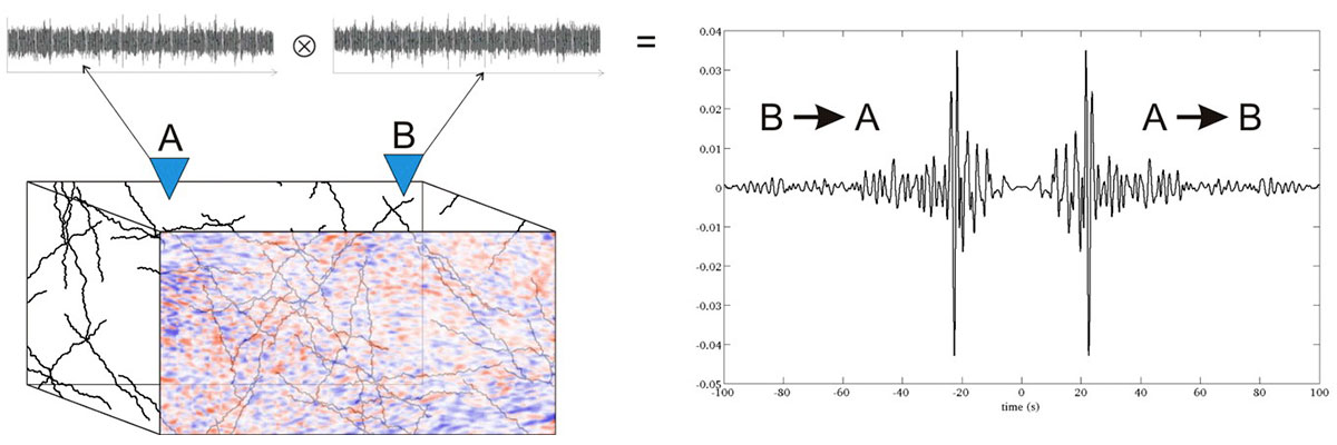
In the past decade, Michel Campillo and co-workers have developed a method using the normal background vibrations (ambient seismic noise) to image the subsurface. Correlations of seismic noise recorded at two stations (sensors) are used to reconstruct the response of the Earth as if one of the receivers acted as a source and the other as a receiver (Figure 1). Using this approach, it is possible to image the subsurface without an active seismic source, in an inexpensive and non-invasive way.
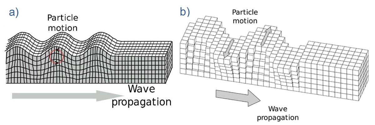
Ambient seismic noise has been studied for decades and it appears that its origin is different for different period bands (Gutenberg, 1958). In general, noise with a period greater than 1 second (i.e. lower than 1 Hz) is due to meteorological conditions such as waves generated by storms on lakes or ocean swell. Noise with a period less than 1 second is mainly due to human activities such as cars and machinery. Seismic noise is dominated by surface waves (e.g. Campillo & Paul, 2003; Shapiro & Campillo, 2004) of which two types can be observed: Rayleigh waves and Love waves. Both have the same propagation direction but the ground motion is different: Rayleigh waves induce ellipsoidal motion in a vertical plane (like ocean waves, Figure 2a), while Love waves induce horizontal motion (Figure 2b). Hence a triaxial seismometer records Rayleigh waves on its vertical and radial components and Love waves on its transverse component. Love waves are shear waves and Rayleigh waves comprise both shear and compressional waves.
An important property of surface waves is dispersion: since the subsurface generally consists of zones of different seismic velocities, waves of different wavelengths travel through different zones and thus travel at different velocities. Since wavelength and frequency are related, dispersion is the effect by which waves of different frequencies travel at different velocities. Typically, seismic velocities increase with depth as the rock becomes less weathered and more competent, and so typically the low frequency waves (travelling through both shallow slow zones and deeper faster zones) are faster than high frequency waves which travel through the slow zones close to the surface.
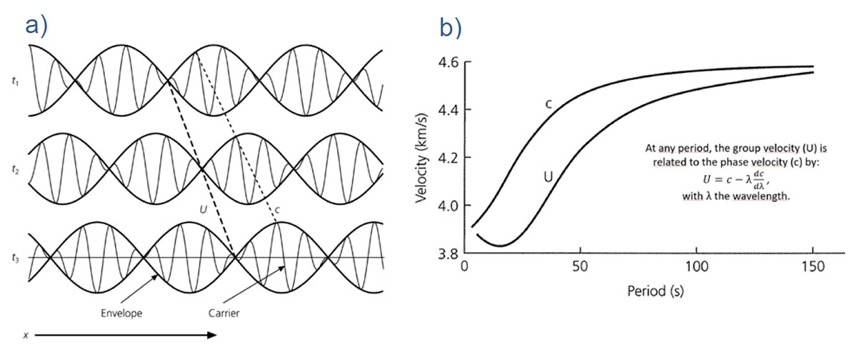
Two types of velocities can be measured: the velocity of the envelope of the signal, called the group velocity, and the velocity of the carrier, called phase velocity (Figure 3). The comparison of a dispersive wave at different travel times shows that the envelope of the signal propagates at a different speed from the carrier. The relationship between the group velocity and the phase velocity implies that if a wave is not dispersive then the phase and group velocity are equal (Figure 3b). In this paper, group velocities are determined using the Frequency Time Analysis (FTAN) introduced by Dziewonski et al. (1969) and average phase velocity using a FK analysis.
Surface waves are recovered by comparing the seismic noise records registered at two different seismic stations. Once surface waves have been retrieved from seismic noise, it is possible to compute tomographic images of the subsurface. Two tools are used to compute shear wave velocity models from surface waves reconstructed with seismic noise. The method of Mordret et al. (2013) is used for 2-D spatial travel-time tomography and that of Sambridge (1999) and Mordret et al. (2014) is used for 1-D depth tomography.
Geological Setting
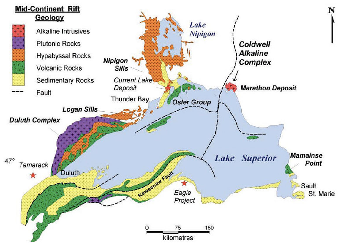
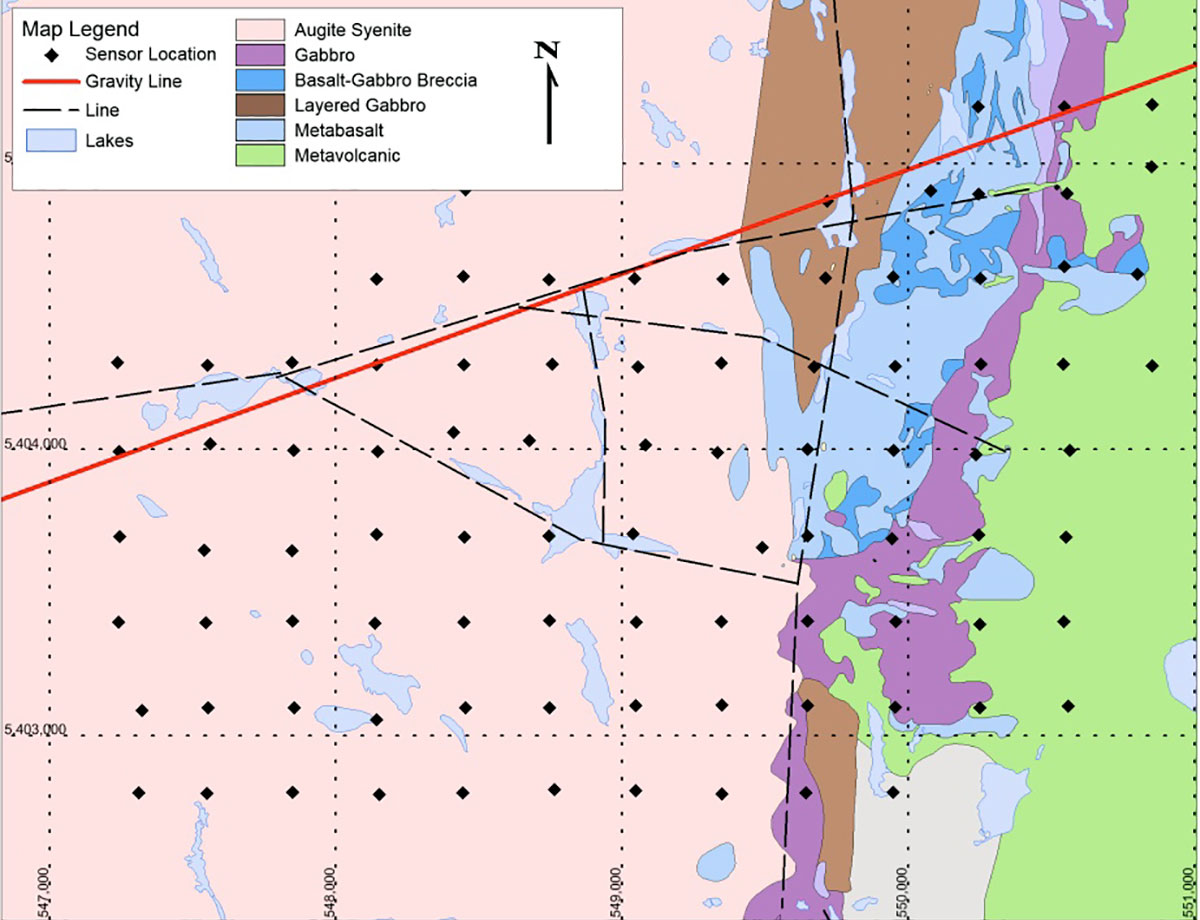
The Marathon deposit is one of several gabbroic to ultramafic hosted disseminated PGE-Cu deposits located around the outer margin of the Coldwell Complex. This Complex is located along the north eastern shore of Lake Superior, near the town of Marathon and is associated with the Midcontinent Rift (Figure 4). It was dated at 1108 ± 1 Ma by Heaman et al., (2007) and between 1107.7 to 1105.3 Ma by Good and Dunning (2018). The Complex, approximately 25 km in diameter, is the largest alkaline intrusion in North America. It is composed of three centres of predominantly alkaline magmatism that intruded the Archean greenstone terrane (Mitchell and Platt, 1977). Centre 1 is composed of Augite Syenite, Quartz Syenite and the Eastern Gabbro Suite. The Eastern Gabbro is composed of numerous gabbroic and ultramafic intrusions of the Metabasalt, Layered and Marathon Series. Geological and geophysical evidence suggests that the Marathon Series intruded along conduits within a large plumbing system beneath the thin flat-lying syenite intrusions.
The mineralization consists of mainly disseminated PGE-bearing Cu-rich sulfides hosted in the Two Duck Lake Gabbro of the Marathon Series. The deposit has dimensions of approximately 3000 m strike length and a variable thickness up to 200 m. Like the intrusion, it dips to the west at about 35 degrees. There are three mineralized zones: the Footwall Zone at the lower contact contains blebby to semi-massive sulfides with low Cu/S ratios; the Main Zone, the thickest and most continuous, is characterized by disseminated interstitial sulfide minerals and the W-Horizon is a zone of high PGE, low S mineralization located at the south end of the deposit. Estimated total proven and probable reserves of 91 Mtonnes at 0.83grams/tonne Pd, 0.24grams/tonne Pt, 0.085grams/tonne Au and 0.247% Cu, containing 3.39 Mounces of combined Pd+Pt+Au and 497 Mpounds of Cu (Murahwi, 2010).
Results
a) Phase I - Noise test
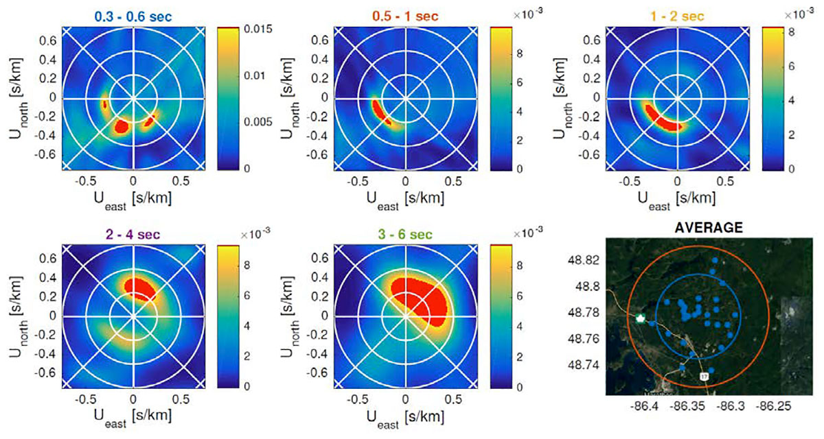
A noise test using an array of 31 vertical component stations was performed to determine the Power Spectral Density and azimuthal distribution of local ambient seismic noise. Use of vertical component stations was dictated by cost and availability of recording equipment for the Phase II survey and allowed only Rayleigh wave analysis to be performed. The station distribution and beamforming results (Figure 6) show that the source of the high-frequency noise lies to the SW and is probably waves on Lake Superior. Low-frequency noise comes from the NE, probably ocean swell on the North Atlantic.
b) Phase II – demonstration of the ambient noise surface-wave technique
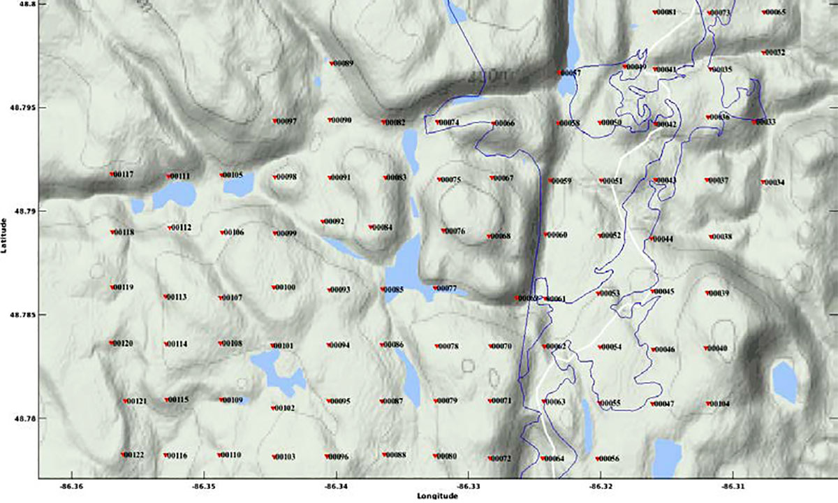
The dataset consists of 26 days of ambient seismic noise recorded over 90 vertical component stations (Figure 7). The nominal distance between the sensors is 300 m.
The Power Spectral Density (PSD) and spectrograms for each individual station show for most stations relatively stable seismic noise with the distinct pattern of oceanic storms at periods above 1 s. In the period band used for the tomography (0.15 - 1.5 s), the noise is made of discrete bursts, probably related to local weather.
Noise cross-correlations and noise source distribution
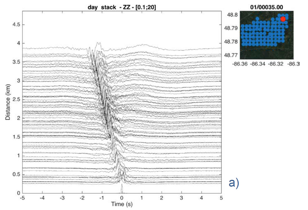
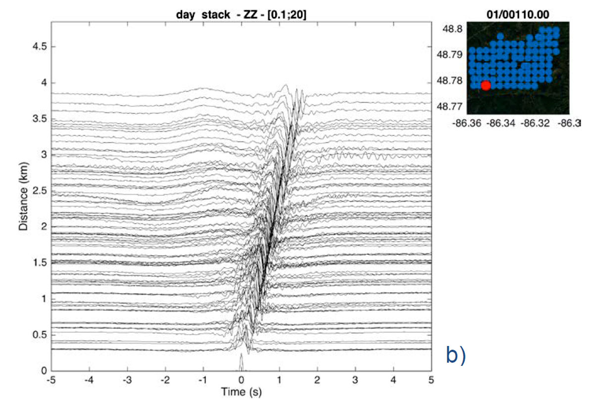
Correlation functions are computed from daily ambient noise records. Signals are first down-sampled from a sample rate of 4 ms to 20 ms and normalized in the frequency band [0.1 - 20] Hz. Figure 8 shows correlations between a reference station (00035 and 00110 acting as a virtual source) versus the other stations in the array. Correlations are sorted as a function of distance from the reference station. Propagation of Rayleigh waves is clearly visible across the array. Most of the noise energy is coming from the southwest (acausal, or negative time, energy on station 00035 correlations and causal, or positive time, energy on 00110 station correlations) in the direction of the Great Lakes (Xu et al., 2017). Some low frequency energy is coming from the northeast. This is confirmed by the beamforming analysis performed in different frequency bands (Figure 6). In the following we will work on the symmetric components of the correlations, i.e., the average of the causal and acausal parts.
Average dispersion curves over the entire network
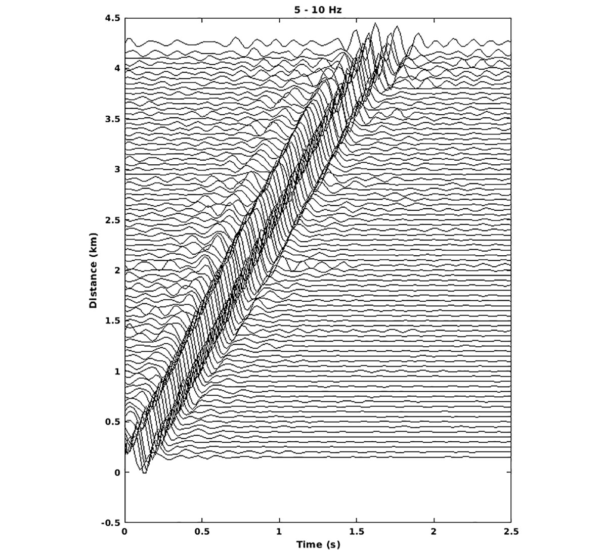
We now build an average seismic section by summing acausal and causal portions of the correlations and binning the correlations in fixed distance intervals (every 50 m). Doing so, we assume that the underlying velocity model is mostly 1D. By stacking the large amount of data in each distance bin, the signal-to-noise ratio (SNR) is highly increased, which allows us to extract the fundamental mode (i.e. the first harmonic) average phase velocity dispersion curve (Figure 9).
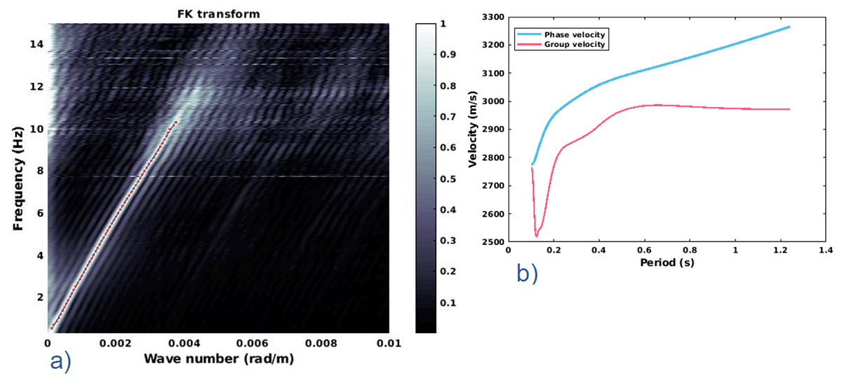
A frequency-wavenumber (FK) analysis of the stack section allows us to accurately pick the average phase velocity dispersion curve for the entire network (Figure 10a). A mean group velocity dispersion curve is then calculated as a derivative of the mean phase velocity dispersion curve according to

where U is the group velocity, c is the phase velocity and ω the frequency. These mean dispersion curves are presented on Figure 10b. We verified that the mean group velocity dispersion curves calculated from FK plots are coherent with the mean group velocity dispersion curves from FTAN picking described later on. The derivation of group velocity from phase velocity involves a differentiation; we smoothed the phase velocity prior to the computation to obtain a stable group velocity dispersion curve. We therefore get an average group velocity dispersion curve which exhibits the correct average velocity value but lacks some variation along the different periods (see Figure 11a).
Group velocity dispersion curve picking and quality control
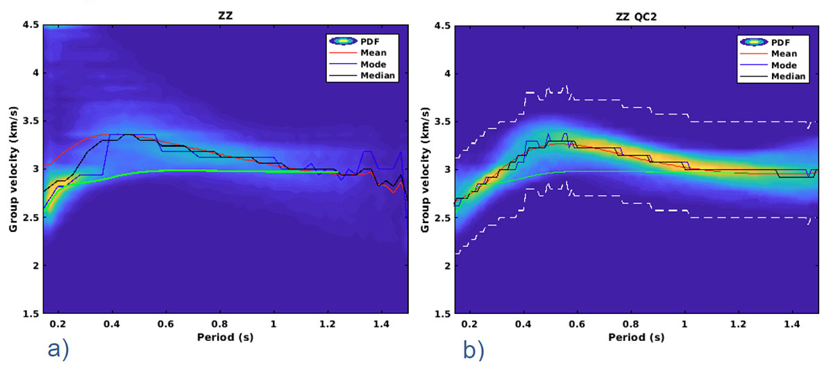
The Rayleigh wave group velocity dispersion curves for the 4005 possible vertical-vertical (ZZ) correlations have been manually picked using the FTAN algorithm. FTAN is a set of narrow Gaussian band-pass filters applied to the correlation. The maximum of the envelopes of the band-pass filtered correlation defines the group velocity dispersion curve for this correlation. We then rejected all the dispersion curves for station pairs separated by less than 900 m to avoid larger uncertainty measurements due to near source effects. Finally, after computing the statistics of all remaining dispersion curves (Figure 11a) we rejected all the dispersion curves for which at least one point falls outside the boundaries defined in Figure 11b, i.e. the values larger (or smaller) than the most probable velocity value (called mode) ± 1 km/s. In Figure 11b, the mode value is shown by the blue curve and the 1 km/s limits by the dashed white curves. The background of the figure shows the probability density function of the Rayleigh wave group velocity dispersion curves, before 11a and after the 11b quality control.
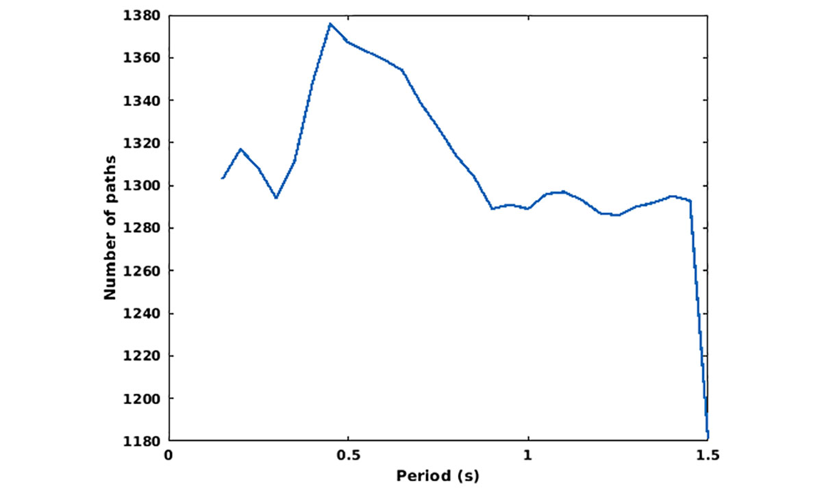
The number of dispersion curves left at each period and used for the tomography is shown in Figure 12. It goes up to 1380 dispersion curves for the period band [0.15 - 1.5] seconds. The number of pairs is limited due to the large (900 m) minimum inter-station distance rejection criterion.
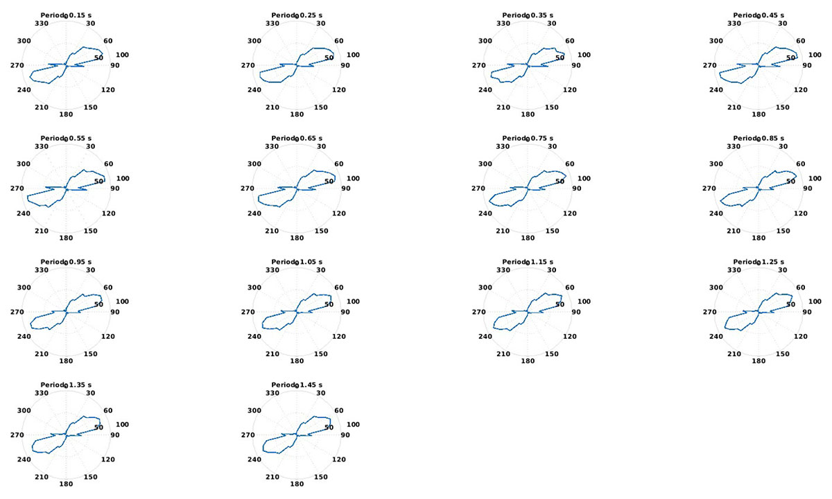
The azimuthal distribution of the Rayleigh wave paths at each inverted period is shown in Figure 13. We can see that the azimuths in the southwest/northeast direction are dominating because the dispersion curves kept during the QC are mostly oriented in this direction, the direction of the main noise sources.
Tomography at different frequencies
The dispersion curves are inverted in the period band [0.15-1.5] seconds (with a regular step of 0.1 s) and regionalized into a regular grid of 100 m by 100 m rectangular cells (in longitude and latitude directions) using the Mordret et al. (2013) approach. Figure 14 shows the results for the Rayleigh wave group velocity maps.
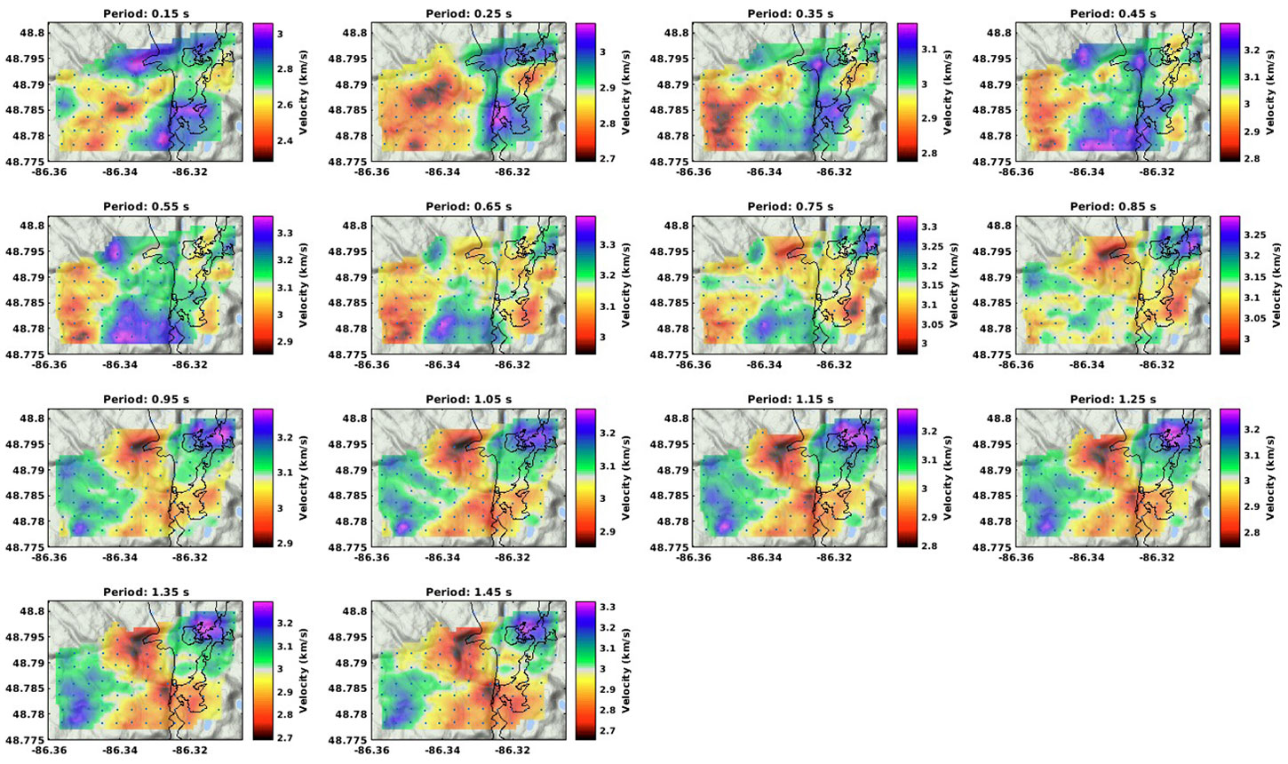
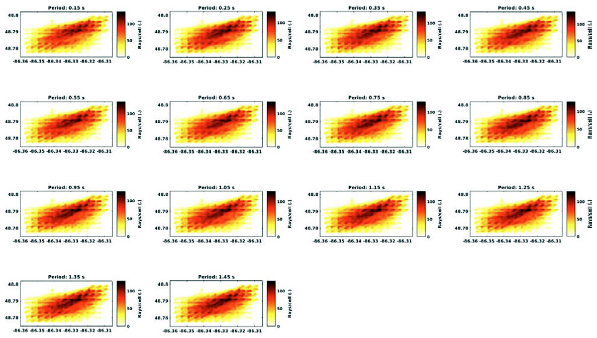
Figure 15 shows the density of rays in each cell of the model at each period for Rayleigh waves. A density of more than 20 rays per cell permits us to achieve a nominal lateral resolution of about 250 m for most of the area, with a minimum resolution of about 500 m at the edges of the area. The density is higher (up to 120 rays per cell) in the middle of the array.
Rayleigh wave group velocity maps show evolving structures with increasing periods. The map at 0.25 s correlates particularly well with the surface extent of the gabbro intrusion.
The full set of group velocity maps describes local dispersion curves at each single cell of the map. These local dispersion curves are then inverted at depth to obtain local 1D shear wave velocity (Vs) profiles. The ensemble of every best local 1D model constitutes the final 3D Vs model. We used a Monte-Carlo approach to invert the dispersion curves at depth because of the strong non-linearity of the problem and the absence of an accurate a priori starting velocity model. This Monte-Carlo approach is based on a Neighborhood Algorithm (Sambridge, 1999) and is described in detail by Mordret et al. (2014). This algorithm has the advantage of exploring entirely the model space using a Voronoï cell discretization while increasing the focus on its most promising areas as the number of iterations increases. The ensemble of best models can be used to estimate some uncertainties on the model parameters. We jointly inverted both Rayleigh group velocity dispersion curves and the mean phase velocity dispersion curve to stabilize and complete the inversion. In total, we inverted 2 dispersion curves for each single cell. These curves are defined in Table 1.
| Wave type | Velocity | Mode | Period (s) | Measurements |
|---|---|---|---|---|
| Table 1: Dispersion curves used in depth inversion for each point of the grid. | ||||
| Rayleigh | Phase | Fundamental | 0.1 - 1.2 | FK |
| Rayleigh | Group | Fundamental | 0.15 - 1.5 | FTAN |
For each dispersion curve presented in Table 1, we define error bars. The error bars of the mean dispersion curves calculated with FK analysis are twice as high as the error bars calculated with FTAN analysis (FK: +/- 200 m/s and FTAN: +/- 100 m/s). This equalizes the contribution of the mean dispersion curves in the inversion. The depth inversion searches for the optimum parameters that minimize the difference between the synthetic dispersion curves and the observed ones. The 1D model is discretized with 3 homogeneous layers with various thicknesses. During the inversion, the P-wave velocity is scaled to Vs using a Vp/Vs ratio of 1.73 and the density is scaled to Vp using the empirical relationship of Brocher (2005). In total, we invert for 5 parameters: velocities in 3 layers and the thicknesses of the 1st and the 2nd layer (Table 2).
| Parameters | Units | Min | Max |
|---|---|---|---|
| Table 2: Parameterization of the local 1D Vs models. | |||
| Vs1 | m/s | 2500 | 3500 |
| Vs2 | m/s | 2800 | 4000 |
| Vs3 | m/s | 2800 | 3800 |
| Depth1 | m | 5 | 700 |
| Depth2 | m | Depth1+100 | Depth1+1000 |
We sampled a total of 21,000 models. The final model is the average of the 1000 best models (with the lowest misfits). This Monte-Carlo technique also allows us to estimate uncertainties for our model as the standard deviation of the distribution of the 1000 best velocity models at each depth. We interpolate the 3-layer 1D models every 1 meter at depth to obtain the final velocity cube.
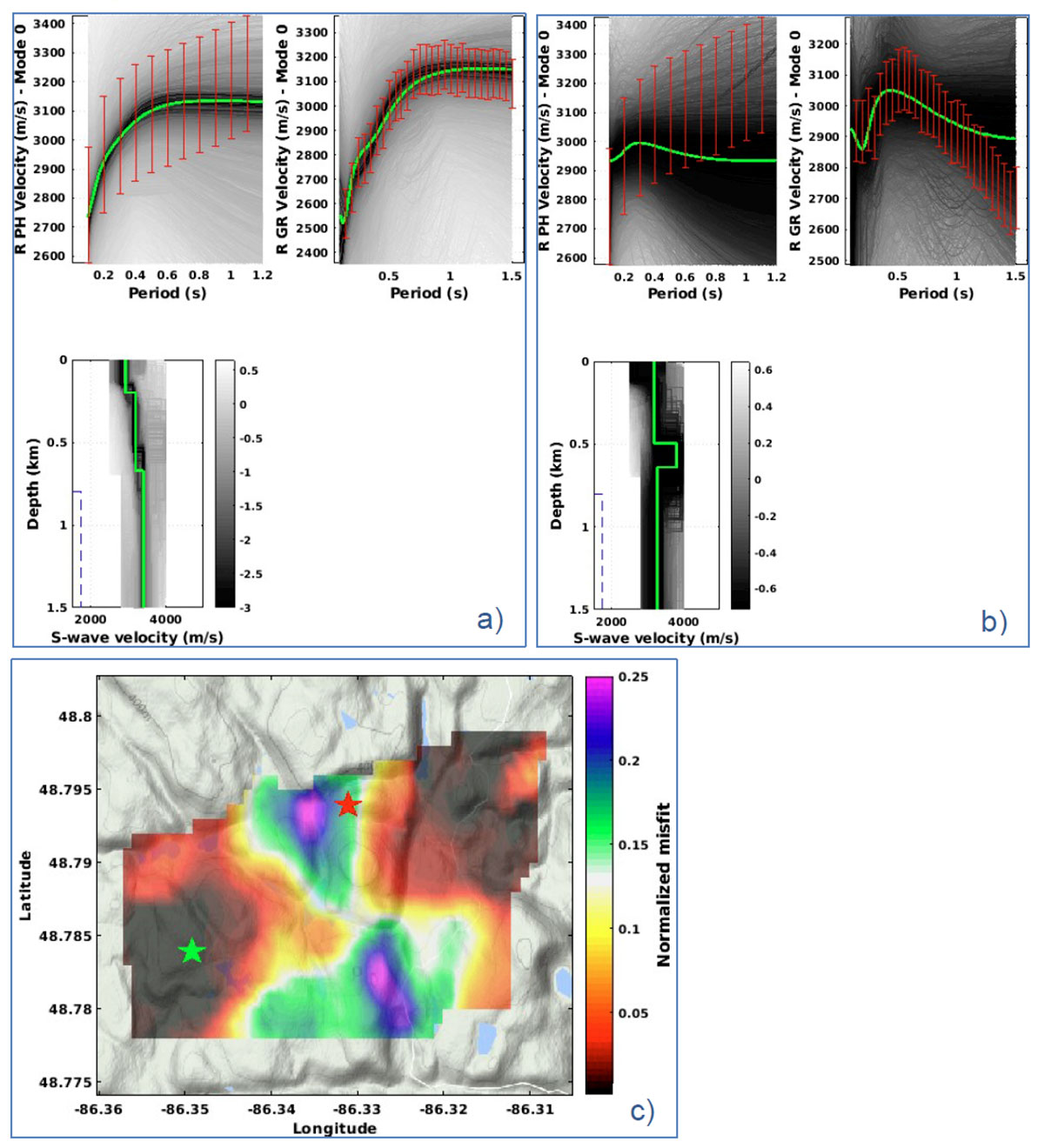
Figure 16 shows two examples of local depth inversion along with the final misfit map. We see that there is a band of higher misfit in the middle of the model (Figure 16c). In this area, the high misfit comes from the poor fit of the average phase velocity that we measured assuming a 1D average velocity model. The dipping slab in this area violates this assumption: the data are sensitive to the thickness of the gabbro intrusion slab and to the material below it, introducing a lower velocity layer which is poorly constrained in terms of velocity. However, the local group velocity is sensitive to the slab geometry. We chose to keep narrow ranges for the inversion parameters to reduce the non-uniqueness of the solutions and avoid over-fitting our results. Although the misfit is larger in these areas, the inverted model parameters are still robust. Given the periods that we used for the inversion, the model is resolved between ~100 m and 1500 m depth.
Final 3D Vs model
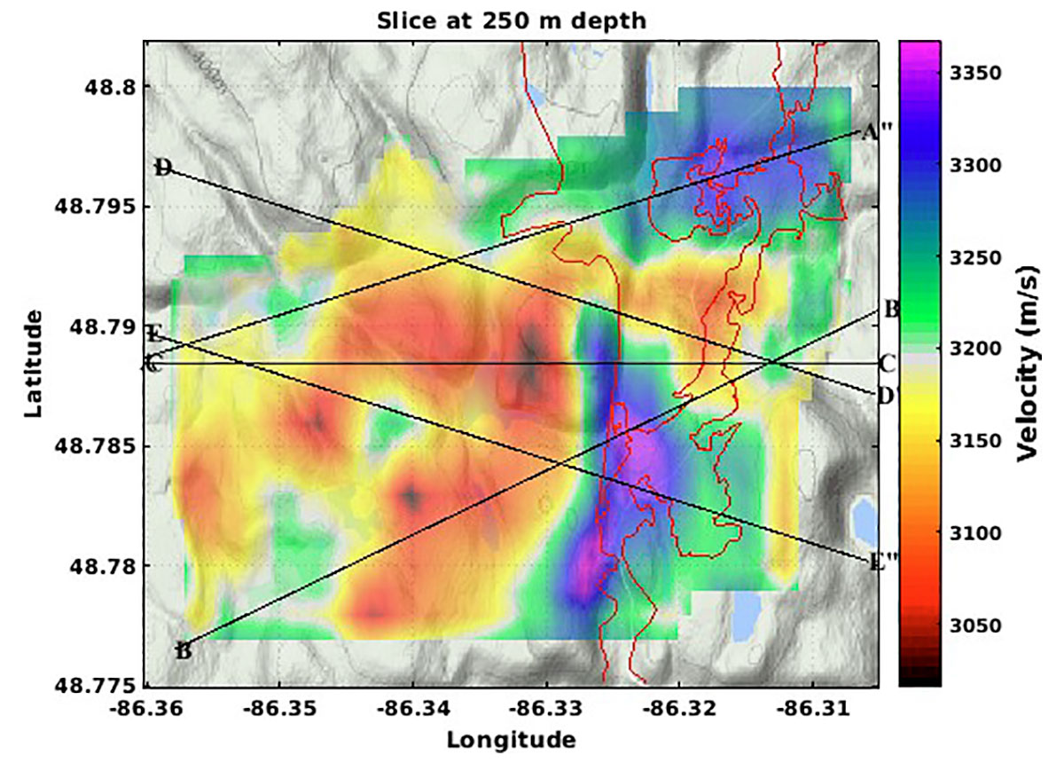
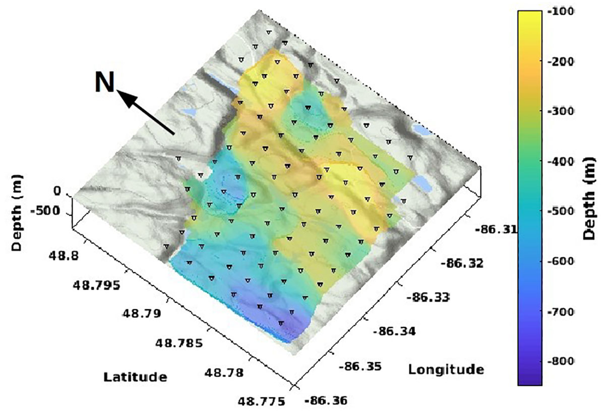
In the following figures we present horizontal (Figure 17) and vertical slices (Figure 18) into the final 3D cube. We observe that the gabbro intrusion slab is well resolved as a higher velocity layer, dipping toward the west. The contact between the upper syenite and lower gabbro intrusion is well resolved but the bottom of the gabbro intrusion is less clear and seems to be picked up by the data only in the middle of the array. However, in this area, the misfit is higher so the interpretation of the slab bottom should be made cautiously.
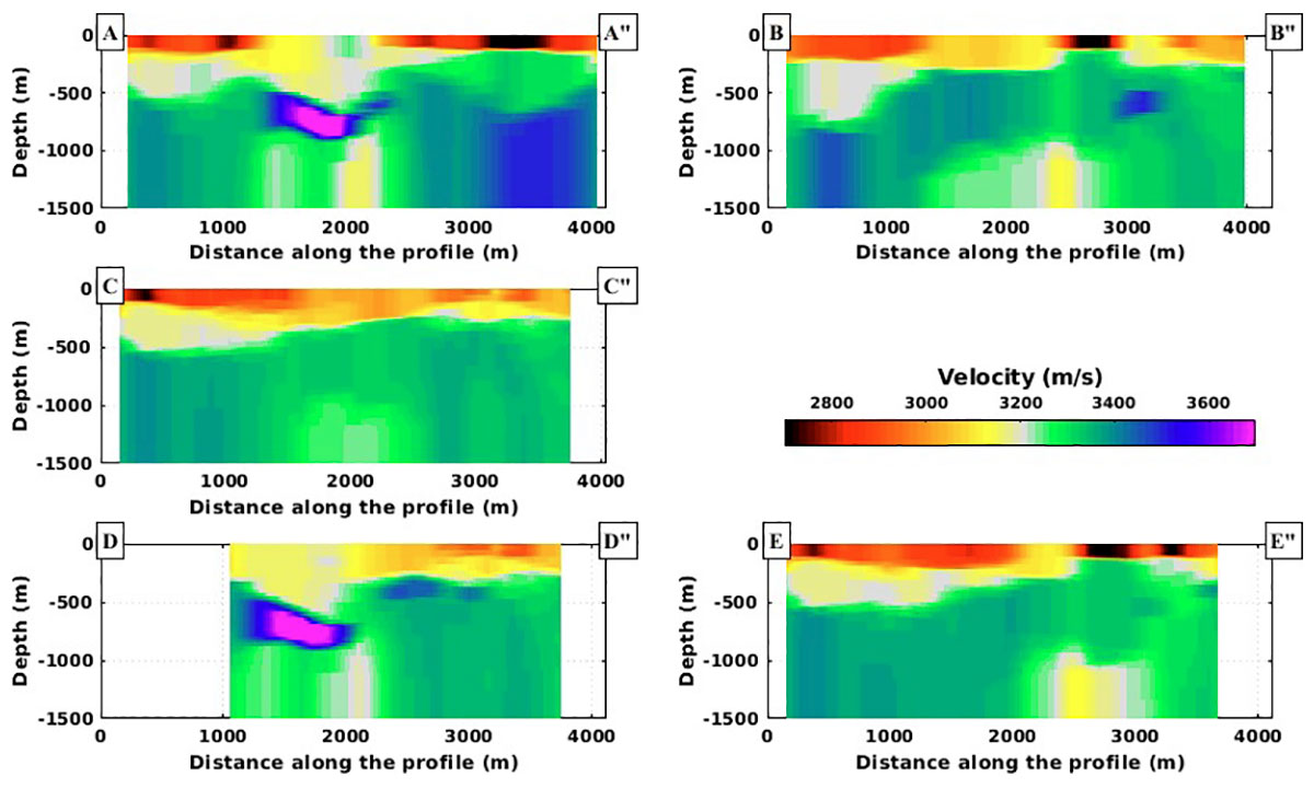
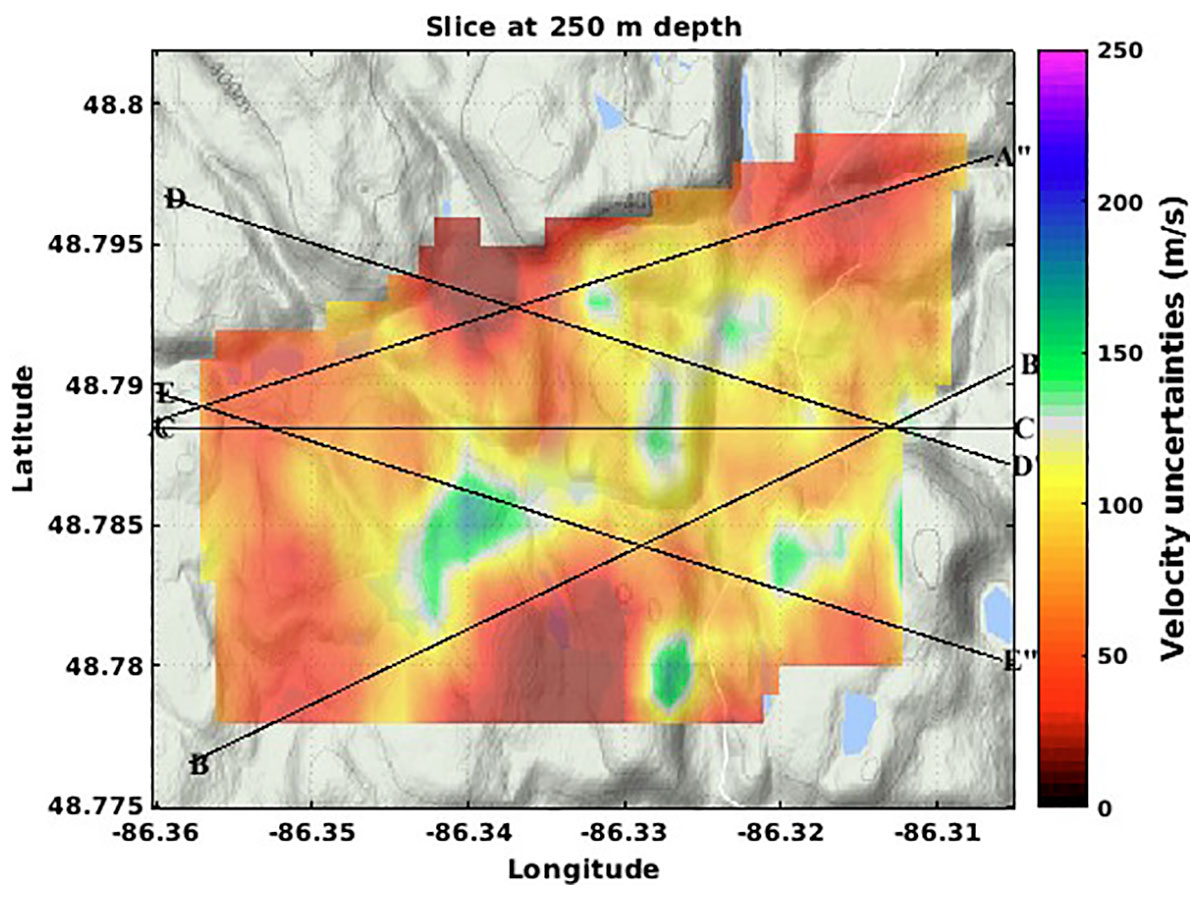
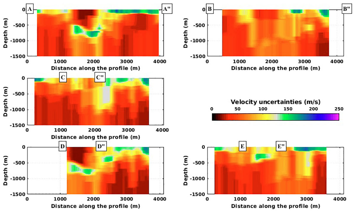
A high velocity anomaly seen on Figure 18 on A and D vertical slices at ~700 m depth is associated with larger uncertainties (Figures 19 and 20) and its true nature is unknown. In order to have a better view of the slab upper surface, we plot the iso-velocity surface at 3250 m/s in Figure 21.
Conclusion
We used 26 days of passive seismic records to retrieve the fundamental mode of the Rayleigh waves propagating across the Marathon area. Most of the noise is coming from Lake Superior.
We jointly inverted local group velocity dispersion curves and the average phase velocity dispersion curve to obtain a robust 3D shear-wave velocity model of the studied area resolved down to 1.5 km. Preliminary interpretation, to be developed in a subsequent paper, is that we were able to image 1) the contact of the gabbroic intrusion which dips to the west, 2) a near-surface layer that could in part be the syenite in the centre of the complex; and 3) a high-velocity zone at ca. 700 m depth that could represent mineralized, olivine-rich gabbro. This interpretation generally agrees with results from the previous core hole drilling program in the survey area.

Acknowledgements
The initial two phases were carried out by a partnership between Stillwater, UGA and Sisprobe and were supported by a Booster Grant from the EIT Raw Materials. The final phase III was one of the main activities of PACIFIC (grant agreement No 776622), a project in the European Union’s Horizon 2020 program. We also acknowledge support from the European Union’s Horizon 2020 research and innovation program for this project.
Related Reading


Join the Conversation
Interested in starting, or contributing to a conversation about an article or issue of the RECORDER? Join our CSEG LinkedIn Group.
Share This Article