Seismic Lithology Prediction: A Montney Shale Gas Case Study

Introduction

In any oil or natural gas development – conventional or unconventional – it is important to understand lithology, as it is a fundamental building block for all reservoir characterization work. Field development is enhanced by the ability to spatially predict different rock-types which in turn have different properties such as fracability and permeability. While petrofacies can be determined carefully for each well in the field using log data integrated with core and sampled data, there is still the issue of predicting lithology between wells. Extrapolating this petrophysical knowledge to seismic data for inter-well lithology prediction can be an important tool for developing the resource, but only if the predicted lithology remains anchored to real-world petrophysical measurements. In this article, we describe a workflow to do just that: apply rule-based petrofacies to seismic to predict lithology, potentially improving well placement and completions in the Montney shale gas play. This work was originally presented at the 2011 CSPG CSEG CWLS Convention.

Lithology Prediction Workflow

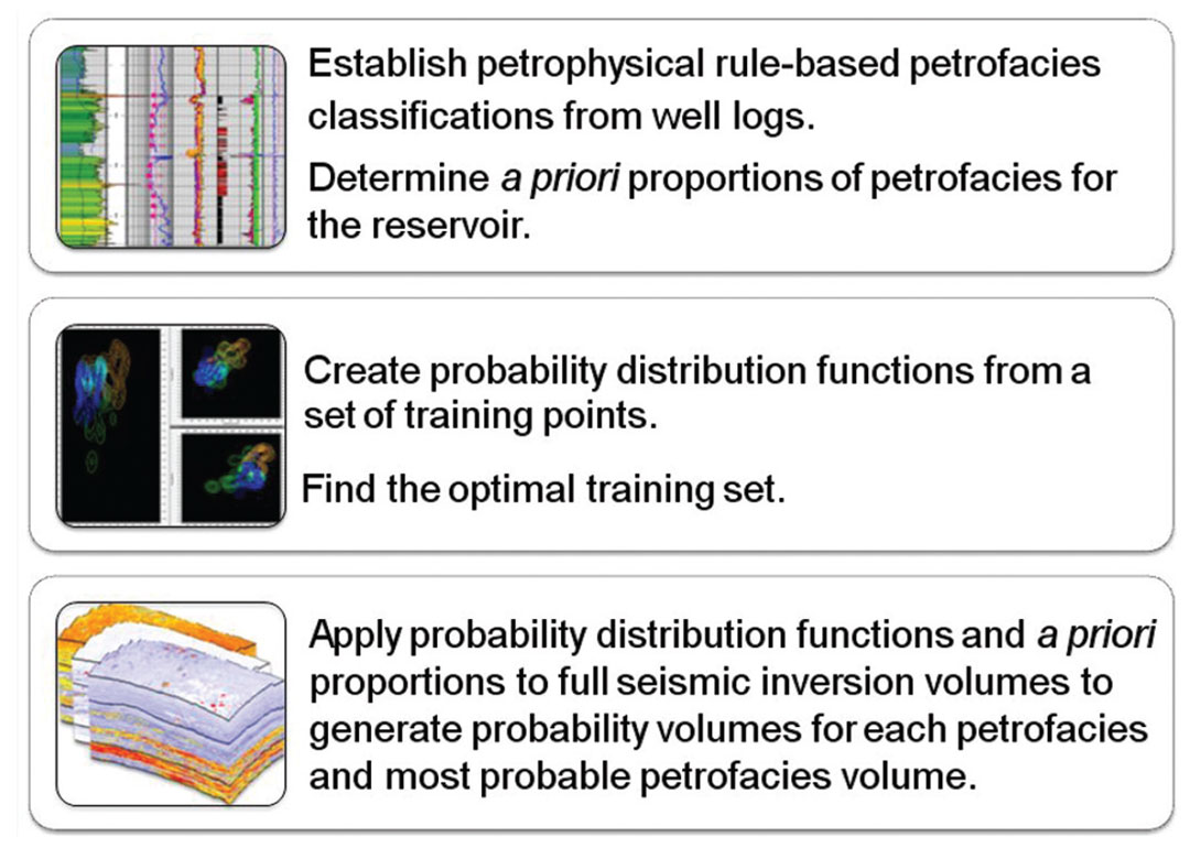
Figure 1 illustrates the lithology prediction workflow in general terms. The approach is to first establish petrophysical rule-based petrofacies definitions, and then demonstrate where – and with what probability – these petrofacies classes are met within a seismic volume (Doyen, 2006 and Coulon et al., 2006). Using elastic parameters from prestack seismic inversion, probability distribution functions (PDFs) are ‘learned’ and then, using Bayesian probability theory, combined with prior knowledge about the reservoir petrofacies proportions to generate probability volumes for each petrofacies and a most probable petrofacies (MPP) volume. The entire process is grounded in careful petrophysical work.

This lithology prediction workflow is designed to predict petrofacies type from seismic inversion attributes, while quantifying the probability of the prediction.

In the following sections, we describe how this lithology prediction was carried out for a Montney shale gas project, and explain the significance of each step in the workflow.

Montney Shale Gas

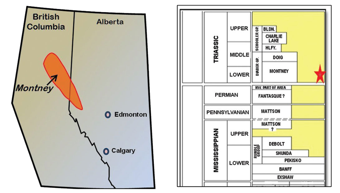
The focus area, in northeast British Columbia, is shown in Figure 2. The Montney formation is pervasive throughout a large area of B.C. trending northwest from the Alberta border towards Fort St. John. One of the most active plays in B.C., the original gas in place is estimated as 450 TCF for this unconventional gas resource (source: B.C. Ministry of Energy and Mines). The Triassic Montney formation (also Figure 2), is approximately 240 million years old and was deposited in a continental-ramp basinal setting (Moslow et al, 1997).

Rule-based Petrofacies Classifications

The majority of the Montney is made up of extremely low permeability highly laminated organic clay, silt, and fine sand (Nieto et al., 2009). Reservoir quality in the Montney is variable. Upper and Lower Montney are deposited in cycles on a scale of tens of meters in thickness, each cycle containing fine scale laminated silts with varying degrees of Total Organic Carbon (TOC.)

These variations in lithology can be predicted by the integration of wireline logs and rock description data using simple cut offs or ‘rules’ applied to the wireline data. The resulting numeric curve assigns a value to each rock type or ‘petrofacies’. Petrofacies are the first and key step in any inter-well lithology prediction. It is recognized that true lithology can only be determined from cores cut in all lithofacies of the reservoir. Cores in a given field, however, are rare, so to leverage the increased data density of wireline log measurements, petrofacies can be implemented. It should be noted that these petrofacies are carefully determined using depth corrected and normalized wireline log data integrated with the actual core and sample data. Several methods are available to define petrofacies (Hook et al. 1994), but the authors’ preferred method is to use simple Boolean rules on log curves to discriminate the different rock types.

The petrophysical work has determined the basic petrofacies or ‘rock-types’ in the Montney. Based on cores, cuttings and thin section work, wireline log responses have been used to predict the basic rock types detailed below. Commonly available log curves were used: gamma ray, resistivity, delta (neutron-porosity – density porosity) and density porosity. In this case study, there were sufficient wells to define four rule-based petrofacies:

The rules use a combination of log responses which respond to various properties of the rock (and are relevant for the specific field area only). The exact script defining Petrofacies 1, for example, is: gamma ray >105 API and resistivity >100 ohm and density porosity ≥4%. Note that Phosphatic and High TOC are distinct petrofacies, but were for this case study merged together into one petrofacies due to the inability of the rules to reliably discriminate between them and also because the small proportion of Phosphatic creates inaccurate statistics. This merging was acceptable to do because the two share similar elastic properties and therefore will not create confusion when using the seismic data for prediction.

Geoscientists are familiar with the gamma ray, which can be used to define sand versus shale. In the Montney however, the gamma ray is responding more to uranium associated with the phosphatic units. These phosphatic units must be discriminated as a separate rock type, as they have intrinsically lower grain density which will need to be accounted for when porosity volumes are created from the seismic at a later stage. The density porosity log has been used to define changes in porosity over the Montney interval. The actual porosity difference between the higher porosity (Upper Montney) and lower porosity, low TOC petrofacies (Lower Montney) is actually quite small in the order of 1 porosity unit as the Lower Montney grain density increases from 2690 to 2730 kg/m³.

Delta, the difference in neutron and density porosity is traditionally used in the industry to indicate sand (clean rock) versus shale, especially in the absence of the gamma ray log. As previously stated, in the Montney the gamma ray is not responding to the shale (clay), but to uranium in the phosphatic layers, meaning it cannot be used to predict clay or shale. Delta is therefore useful in the Montney to detect clean (very low clay) silty intervals such as the turbidites seen in the Lower Montney

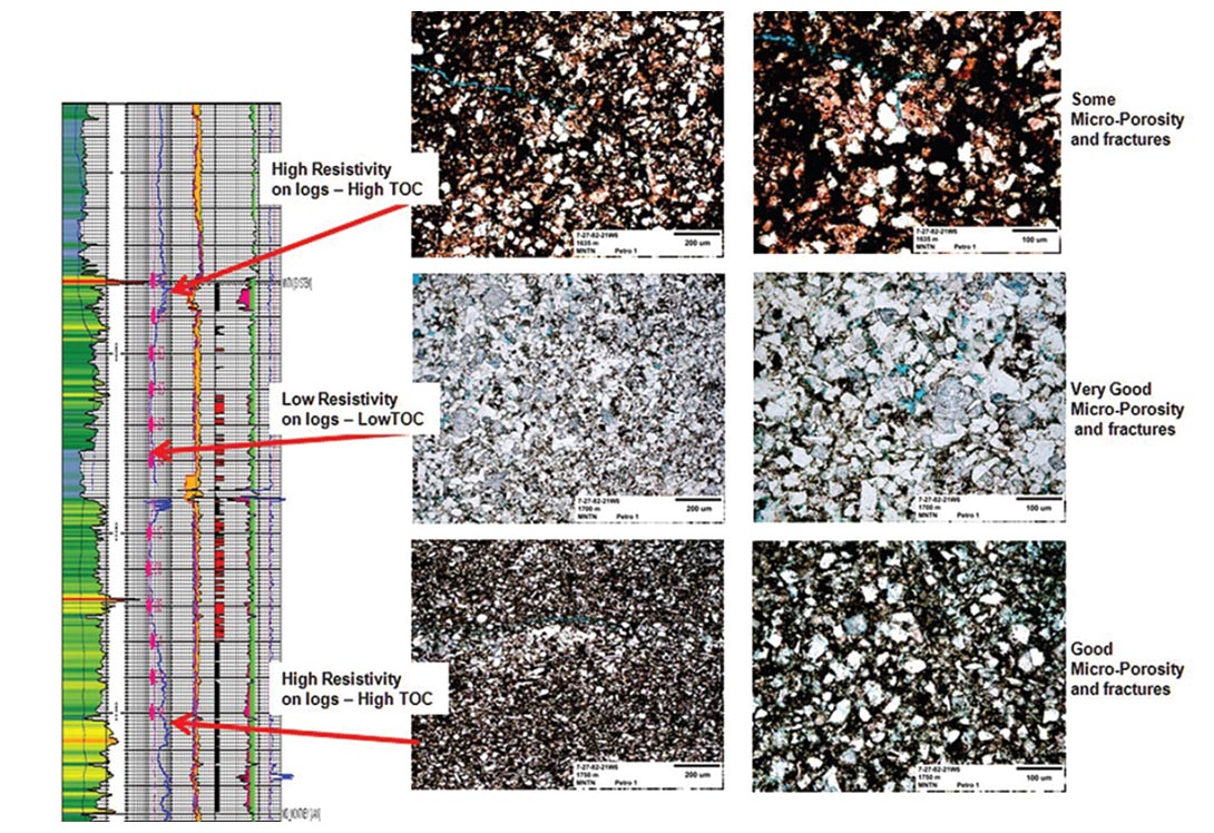
The resistivity log has been used to identify how much organic material is present in the rock. Figure 3 below illustrates the difference between the high and low TOC petrofacies (Petrofacies 1 and 4) in the Upper Montney. The low TOC in the rock leads to higher permeability, requiring slightly different completion technology (Nieto et al., 2009). The same is true for the Lower Montney, largely comprising Petrofacies 2 and 3 which both have low TOC. Petrofacies 4, 3 and 2 and the main development targets in the area. Figure 4 demonstrates the relationship between resistivity and measured TOC content of the rock.

In this Montney case, these four rule-based petrofacies were applied to the four wells available over the 3D seismic survey area for use in the calibration and quality control (blind testing) of the lithology prediction workflow.

The A Priori Petrofacies Proportions and Bayes’ Theorem

Once the petrophysical rule-based petrofacies definitions have been established, the proportion of each petrofacies for the reservoir must be determined. This is a calculation of the proportion of each petrofacies in the well log data.

The petrofacies proportion is a priori information that will be incorporated in the Bayesian classification stage of the workflow to generate petrofacies probability volumes. Why? For finite and noisy data such as a seismic survey, many possible models will fit the data. However, we know that some models are more probable than others. Bringing in this prior knowledge about petrofacies proportions allows the solution to be weighted towards what we know are more realistic models. Bayes’ theorem provides a way to incorporate this prior knowledge by weighting this initial a priori proportion with a distribution function to compute probability for each petrofacies.

Assuming there is a good understanding of the depositional model, the a priori proportions may be adjusted manually to address known biases in the sampling. For example, proportions may be adjusted to take into consideration that well data may over-represent prospective locations in a reservoir. It is also possible to incorporate spatial trends in the petrofacies proportion, although this was not needed for this case study.

Elastic Parameters Provide a Common Language

It is helpful to consider both the petrofacies classes and the seismic in terms of elastic parameters. For the petrofacies, this means using sonic, dipole sonic, and density logs. For the seismic, it means performing prestack inversion to generate Pimpedance (Z_p), S-impedance (Z_s), density, and associated elastic parameter volumes LambdaRho, MuRho, Poisson’s ratio, and Young’s modulus which can all be derived from the two impedances and the density. In this case, deterministic simultaneous elastic inversion was run on near (0-12 degrees), mid (12-24 degrees), and far (24-38 degrees) angle stacks from a 3D seismic survey. It is important to note that the angle stacks were assembled from conventional P-wave wide azimuth gathers, processed with an Azimuthal-AVO-compliant flow. Estimating density from the seismic is often difficult, and in this case, multi-linear regression analysis (via multi attributes analysis software) was used to bring added stability to the density volume.

Probability Distribution Functions

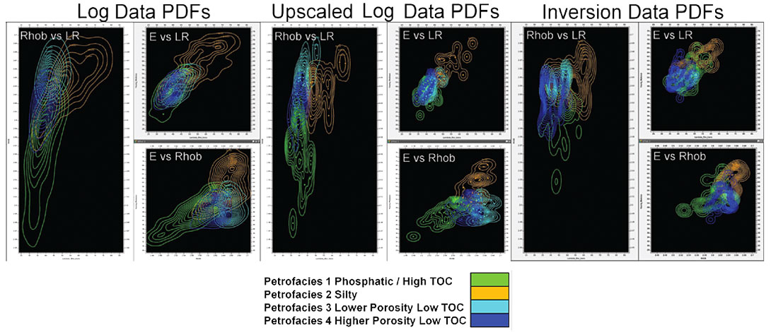
To relate the petrofacies to the seismic data, one could use a basic cross-plot method: cross-plot elastic parameters from the logs, display the data points in colour according to petrofacies and define cutoffs for the petrofacies by drawing a polygon in crossplot space. Then map only the data points from the selected polygon on the inversion volume. In other words, define isolated areas in cross-plot space that represent petrofacies.

The problem with this simple cross-plot mask approach is that the result depends critically on the size of the arbitrarily defined polygon when petrofacies zones start to overlap in cross-plot space. Instead of a sharp cut-off for the lithology criteria, a natural extension of the traditional cross-plot approach is to define a probability distribution (one may visualize a sort of contoured polygon in cross-plot space; Figure 6).

PDFs are built by smoothing the data points in the cross-plot with an operator. The user controls the size of the operator, and hence the smoothness of the function. The operator transforms discrete points into a continuous density function. This approach is called non-parametric statistical classification. (Please see Appendix for more details.)

Further, performing this computerized classification scheme allows one to make use of higher-dimensional cross-plots. While basic cross-plots enable evaluation of relationships between two attributes, 3D cross-plots display inter-relationships among three attributes. It is very difficult to draw 3D polygon zones manually (try juggling three inter-connected cross-plots). Using PDFs provides a way to handle this automatically, enabling two, three or more inversion volumes in the analysis. In this case study we decided to use three however if beneficial more dimensions can be used.

Find the Optimal Training Set: Well Logs, Upscaled Well Logs, or Seismic Inversion

PDFs are created based on a set of training points. This step of the workflow is actually a detailed investigation to find the optimal training set, and may include iterations to revisit the petrofacies rules and/or the a priori proportions of the previous step, if needed.

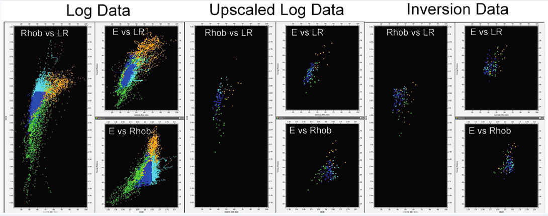
There are three possible sources for a training set of data points that can be used for ‘learning’ a probability distribution: the well log data, the well log data upscaled to seismic scale, or the seismic inversion at the well locations (Figures 5 and 6). It is important to keep in mind the sources of relative uncertainty in these training sets. For the well log data the main uncertainty is due to the fundamental restriction of using elastic logs (because of overlap between petrofacies in cross-plot space). For the upscaled well logs, there is increased uncertainty from the loss of resolution (this can be observed in Figure 7 by comparing the input log to the upscaled log). Finally, for the inversion results, there is even more uncertainty from the data quality and the quality of the seismic inversion. By using PDFs, one can quantify the uncertainty of each training set (via the confusion matrix QC, described below). This is a noteworthy improvement from the basic cross-plot method.

While PDFs generated from the well log data cannot be applied to the seismic volumes (because log data are not at the same vertical sampling scale as the seismic wavelength), such PDFs are useful as a baseline reference for what can be achieved with the other training sets. As well, various combinations of elastic parameters are investigated at this stage to see which gives the best discrimination of the petrofacies in cross-plot space. In this Montney study, for example, density (Rhob), LambdaRho (LR), and Young’s modulus (E) were found to be the most suitable elastic attributes for discriminating the petrofacies. PDFs from the inversion training set were used.

Quality Controls

The PDFs from the various possible training sets are computed and evaluated using several QC measures including visual examination of the separation of petrofacies in cross-plot space (Figures 5 and 6), comparison of actual and predicted lithology at well locations (Figure 7), and confusion matrix results (Figure 8).

1. Separation in Cross-plot Space

In addition to visual examination for separation of the petrofacies in cross-plot space, independent quantitative measures of separability (the degree of separation or overlap in cross-plot space, for the given data) and confidence coefficient (a measure of the confidence that can be placed in the statistics) are also used as QCs of the PDFs.

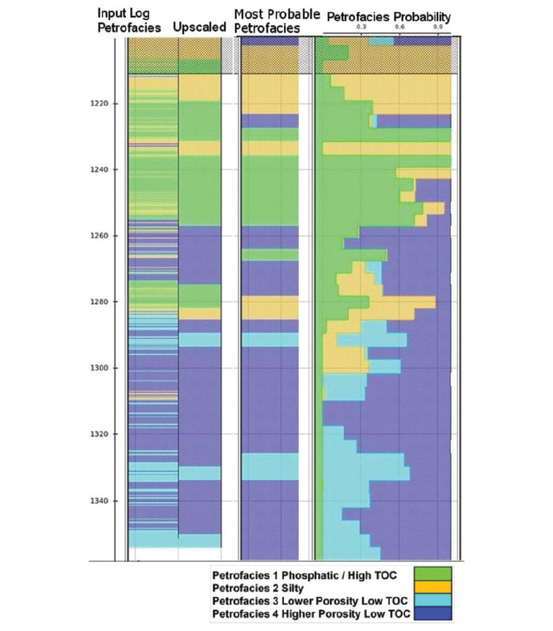
2. Actual Compared to Predicted Lithology

At each well location, the Bayesian classification process is applied to the inversion volumes to generate probability and MPP, and these are compared to the actual petrofacies log. Figure 7 shows this QC for Well 3. The middle track – the ‘most probable’ petrofacies from seismic – demonstrates good agreement with the actual petrofacies determined from logs in the well in the left hand track. Note that the probabilities can also be helpful indicators of where there may be indefinite or mixed lithologies.

3. Confusion Matrix

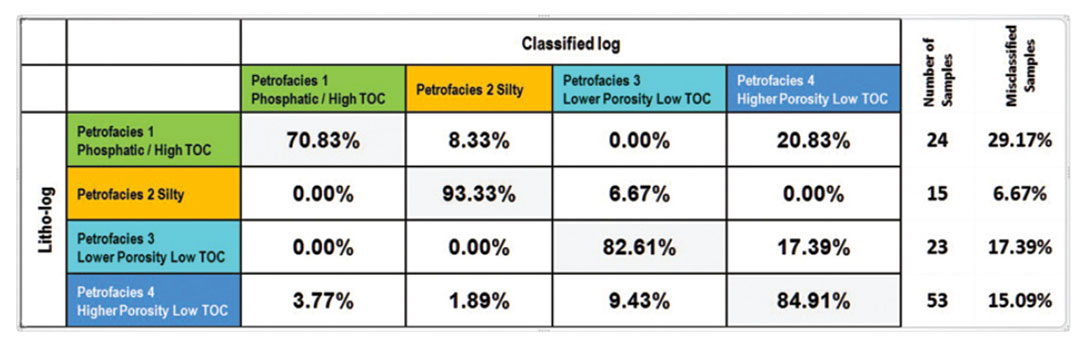
If the prediction process had worked perfectly, the actual and predicted petrofacies would be identical. Any colour mismatch is an error or “confusion” between the petrofacies. The mismatch for the whole process is summarized in the confusion matrix (Figure 8). The confusion matrix is a key QC for the prediction process, answering the question, “How often do we correctly predict a petrofacies?”

The diagonal elements show the success rate of the prediction process for each petrofacies. For example, Petrofacies 2 (Silty) is very well resolved: when the actual petrofacies log is silt, the classified log predicts silt 93.33% of the time.

The off-diagonal elements in the matrix quantify what has been confused with what. For example, Petrofacies 3 (Lower Porosity Low TOC) was confused with Petrofacies 4 (Higher Porosity Low TOC) 17.39% of the time. To improve this, one could revisit the smoothing parameters within the PDF calculation, the initial a priori reservoir proportions, or possibly the petrofacies rules or the number of petrofacies. The number of samples is also listed in a confusion matrix analysis, to show whether the results are statistically meaningful.

In summary, a good quality prediction is indicated when diagonal elements of the confusion matrix are large and off-diagonal elements are small.

Probability Volumes and Most Probable Petrofacies Volume and Interpretation

Following proper QCs at the well locations, the Bayesian classification can then be applied to the full seismic volume to generate probability volumes for each petrofacies, and an MPP volume.

A 2D line through the well locations, extracted from the probability volume for Petrofacies 4 (Higher Porosity Low TOC) is displayed in Figure 9. The colour scheme represents probability of occurrence of this petrofacies. Note the high probability of Petrofacies 4 predicted in the Upper Montney at Well 1, for instance.

One may use probability volumes to detect probable sweet spots within the best petrofacies layer.

Figure 10 shows the 2D line extracted from the MPP volume. It should be noted that the MPP volume should not be interpreted alone, but should always be considered in concert with the petrofacies probability volumes because the MPP does not convey the uncertainty. For example, in the case of four petrofacies, it is possible for one to be classed ‘most probable’ with a probability as low as 25.1%.

In this Montney example, the lithology prediction does show lateral variations, indicating that the geology is not completely homogeneous as is sometimes assumed in the Montney formation.

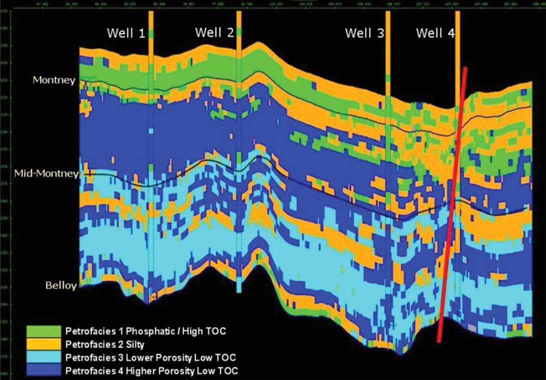
For instance, more Silt (Petrofacies 2, orange) is predicted near Well 4, compared to Wells 1 and 2. This is evidence of cementation associated with the fault that the well penetrates. This cementation has a threefold effect. Firstly, the velocity is higher and the porosity lower in this rock type. Secondly, the resistivity is higher. Lastly, the gamma ray response is lower due to increase of the calcitic material. These responses combine in the rulebased classification to identify Petrofacies 2, Silt. This silty unit, commonly found in the Lower Montney is thought to be derived from coarser sediment flow into the deeper basin in the form of turbidites and is an important unit for development. Consequently, the prediction of the calcitic material associated with the fault really requires another set of rules to discriminate it from the Silt Petrofacies. This lithology difference was well understood in this case study, and demonstrates that a good geological understanding is essential in order to correctly interpret the MPP volumes. The seismic lithology prediction is doing a good job of picking up the lateral variations, helping the interpreter to assess the extent of the lateral and vertical influence of the faulting.

The presence of Petrofacies 1 – the phosphatic layer – at the top of the Montney is important as it acts as a barrier to fracture height growth during fraccing. Hence, predicted variations in thickness of this petrofacies are of importance.

Further, the lithology prediction allows one to visualize and map the extent of the most prospective zones – Petrofacies 4 in the Upper Montney – the high porosity, low TOC petrofacies and Petrofacies 3, the slightly lower porosity, low TOC petrofacies in the Lower Montney.

Ideally, the results should also be validated with a blind or new well, if available. To date, the predictions of the rock quality and distribution of the petrofacies from the 3D seismic have been validated to the extent that the model has been used for horizontal drilling in the Montney (several horizontal wells have been drilled since this work was completed in spring of 2011).

Also, since the inception of this work there have been additional wells, logs, and core data. Consequently, some refinements to the number of petrofacies predicted in the initial model have been made and indicate that it is now possible to identify as many as six petrofacies types, thus increasing the heterogeneity prediction capability of this workflow. Typically, geomodels such as this are ‘evergreen’ and will be updated regularly as more data become available.

Conclusions

Initially this Montney case study began with prestack seismic elastic inversion to evaluate lateral continuity of the reservoir quality. The good match between the wells and the inversion indicated that the interpretation could be further enhanced by carrying on to lithology prediction.

Variations in lithology within the Upper and Lower Montney require the establishment of rule-based petrofacies. In this study, four petrofacies or rock types were defined from rules using commonly available logs. Using the rule-based petrofacies definitions and multiple elastic parameters from the prestack seismic inversion, Bayesian classification provided a means for petrophysical properties to be extrapolated throughout the 3D data volume for the Montney, yielding inter-well petrofacies predictions and associated probabilities.

The predicted petrofacies and their respective probabilities from this workflow provide a building block for reservoir characterization work: populating the ‘Static’ Earth model with petrofacies is the first step in determining better porosity, permeability and saturation calculations prior to using in the “Dynamic” Earth Model for reservoir simulation. Each of these petrophysical properties uses the petrofacies as a discriminator to select the correct equation for calculation throughout the volume.

These volumes are used to plan well locations in the Upper, Middle and Lower Montney formations and when drilling the wells to ensure that the well path stays in the desired target zone. Furthermore, identification of any petrofacies changes along the wellbore is useful additional information for completion planning.

Acknowledgements

The authors wish to thank Canbriam Energy Inc. and CGGVeritas Multiclient Canada and Alaska for permission to publish this case study, and Robert Bercha, Graham Carter, Jon Downton, Jan Dewar and others for their valuable suggestions and assistance in preparing this article.