Noise reduction by structure-and-amplitude-preserving multi-channel deconvolution

Abstract

We pose seismic noise reduction as an inverse problem. The clean data are obtained by minimizing a cost function that uses a priori information about the spatial continuity of reflectors. The optimization problem is solved by introducing a smoothing operator that reduces the difference between adjacent traces along seismic events. The smoothing operator is estimated from the data using FX (temporal frequency and space) domain prediction filters. In essence, we propose a seismic de-noising strategy that operates as a multi-channel deconvolution with the addition of dip consistent spatial smoothing.

We show that the proposed method can preserve subtle structural information, residual moveout and amplitude-versusoffset signatures. We test the algorithm with gathers from the Marmousi data set and a real dataset from the Western Canadian Basin.

Introduction

Noise-reduction is important in seismic data processing since noise compromises our ability to depict the earth interior. Noise can be classified into coherent noise and incoherent noise according to its predictability. Coherent noise can be predicted using model-based approaches. For example, multiples after NMO exhibit parabolic moveout and therefore the parabolic Radon transform can be used to model the multiples in the transform domain. The multiples are transformed back to the data space and finally, are subtracted from the original data (Hampson, 1986; Sacchi and Ulrych, 1995; Ng and Perz, 2004). A similar idea can be used to remove incoherent noise. The difference is that in incoherent noise reduction we try to model and keep the coherent signal. The residuals are an estimate of the incoherent noise. Examples of incoherent noise reduction are the well-known FX deconvolution and FX projection filtering algorithms proposed by Canales (1984) and Soubaras (1994), respectively.

It has been shown that regularized migration/inversion using a priori information about the underlying reflectivity model can yield high quality images of the subsurface (Wang et al., 2005). In this paper, a similar idea is used to design an algorithm for multi-channel signal-to-noise-ratio enhancement. We assume that seismic events are spatially predictable within a gather and use FX domain prediction filters to enforce spatial continuity of the reflectivity. The idea leads to a constrained least-squares problem in preconditioned mode. It is important to stress that since FX domain prediction filters contain structural information, there is no need to pick horizons (Prucha et al., 2002) to form dip-friendly constraints.

Methodology

We start our discussion with the following simple equation

where the i-trace ( d_i^obs (t) ) is represented via the convolution of the reflectivity ( r_i (t)) with a wavelet plus additive noise ( n_i (t) ). Equation (1) can be transformed to the frequency domain

Equations (1) and (2) provide a data constraint for the reflectivity in the time and frequency domains, respectively. Now we make the assumption that the reflectivity is laterally continuous. In other words, we do no expect high trace-totrace spatial variability. The lateral continuity of the reflectivity in the presence of structural dip can be represented by a prediction filtering equation (Canales, 1984):

where P_i (ω), i = 1,L, are the coefficients of the spatial prediction filter of length L. The auxiliary variables Z_i (ω) can be interpreted as reflectivity prior to undergoing spatial filtering. Equation (3) stresses the fact that the spatial variability in the window of analysis can be modeled by events with constant dips (Canales, 1984). After combining equations (2) and (3) we obtain

It is now possible to write equations like (4) for all frequencies leading to the following expression in matrix form:

We now introduce the Fourier operator, F, that transforms data from the TX (time-space) domain to the FX (frequency-space) domain. In addition, we introduce the inverse Fourier transform, F^-1 , to transform data from the FX domain to the TX domain. Using forward and inverse Fourier transforms, we can express equation (5) as below:

where d^obs is the time domain data, W̃ represents the time domain convolution matrix of the wavelet, z is the time domain representation of the vector Z , and n is the time domain noise. The method of conjugate gradients (CG) (Hestenes and Steifel, 1952) is used to estimate the vector z by minimizing the following cost function

where the first term on the right side is the L2 norm of the residual, the second term is the L2 norm of the vector of unknowns z. The scalar µ is a trade-off parameter used to control the degree of fitting. We will ignore the trade-off parameter (i.e., µ = 0 ) and rely on the number of iterations of the CG method to control the misfit (Hanke and Hansen, 1993). Note that when we minimize the cost function (7) there is no need to form explicit matrices. We implicitly compute matrix times vector multiplications. This strategy was also discussed in Wang and Sacchi (2005) and described in the following paragraph.

The CG method minimizes the cost function via a sequence of steps (Claerbout, 1992). In each step two linear operators are required; a forward operator, L = W̃ F^-1PF , and its adjoint (or transpose), L^T =F^-1P^TF W̃ ^T . The symbol (.)^T indicates operator transpose. Let’s consider an arbitrary vector x and study how one can implement the forward operator, Lx = W̃ F^-1PFx . First x is transformed to the FX domain (i.e., Fx). Then prediction filtering is used to apply dip-preserving smoothing (i.e., PFx). The results are transformed back to the TX domain (i.e., F^-1PFx). Finally multichannel convolution with a wavelet is applied (i.e., W̃ F^-1PFx). The adjoint operator ( L^T = F^-1PTF W̃ ^T ) is implemented in a similar fashion but convolution ( W̃ ) is replaced by its adjoint ( W̃ ^T ), crosscorrelation (Claerbout, 1992), and the prediction filter ( P ) is replaced by the adjoint prediction filter ( P^T ).

Once the solution vector z is found, the predicted (clean) data are estimated by the following expression

It is important to mention that we have introduced spatial preconditioning into our model (equations (6) and (7)) via the FX domain operator P. This is similar to use low-pass operators to precondition inverse problems as suggested by Ronen et al. (1995) and Fomel and Claerbout (2003). The generic idea of preconditioning is to filter the model with an operator that preserves desired features in the model. The desired features come from a priori information about the model. In the case of multi-channel deconvolution, we assume a laterally coherent reflectivity model. Note that lateral smoothing operators including FX prediction filters can smear sharp structures like faults. Our method is less likely to introduce undesired amplitude smearing because the prediction filter is used as a preconditioner to stabilize the multichannel deconvolution. In classical FX filtering, on the other hand, the prediction filter operates directly on the data, leaving little room to avoid amplitude smearing.

Wavelet estimation

In the proposed method we regress multi-channel data by fitting a model that requires the seismic wavelet and FX prediction filters. We estimate the seismic wavelet using the classical white reflectivity assumption and decide its phase based on a phase assumption (minimum phase, zero phase or zero phase plus a phase rotation). The amplitude spectrum of the wavelet is estimated from the data using the average autocorrelation of the traces in the window of analysis followed by smoothing.

Estimation of the prediction filter

Ideally prediction filters should be estimated from the unknown reflectivity. This poses a non-linear problem. To avoid this difficulty, we estimate prediction filters directly from the data. The strategy is justified because data and reflectivity portray similar spatial continuity. The prediction filters are estimated by solving the classical linear prediction equations in forward and backward prediction modes. Once we have solved for forward and backward prediction filters we combine them to form a unique operator P for all frequencies. In essence, the operator is used to incorporate dip-preserving smoothing for adjacent traces. If one replaces P by the identity operator ( P=I ), there will be no dependency between traces and the multichannel deconvolution will degenerate into conventional single trace deconvolution. In our new method trace-to-trace variations (jitter) resulting from single channel deconvolution are removed by the spatial filtering introduced by the operator P.

Synthetic examples

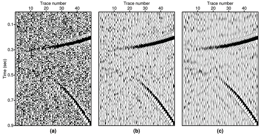
In the first example, we apply and compare the proposed method with FX prediction filtering (Canales, 1984) using a simple multi-channel synthetic dataset. As shown by Figure 1, the input data have two events with residual moveout and strong Amplitude Variation with Offset (AVO). As we expected, both Canales’s methods (1984) and the proposed method can preserve the residual moveout. Careful comparison shows that the new method provides more coherent amplitude along the offset direction than the standard method (Canales, 1984).

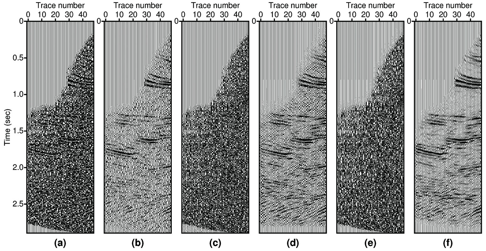
We also compare the performance of the two methods (Canales’s method (1984) and the new method) using a CMP gather extracted from the Marmousi dataset (see Figure 2a). For testing purposes, we applied NMO to the original gather. The NMOcorrected gather was contaminated with random noise. Note that the seismic events in this example are more difficult to predict than those in the previous example due to the complexity of the Marmousi model. In spite of the complexity of this gather, the new method was able to reduce the noise without destroying the amplitude signature. In particular, the new method provides better focusing of events in the time window from 2.0 second to 2.5 second (see Figure 2d).

Real data example

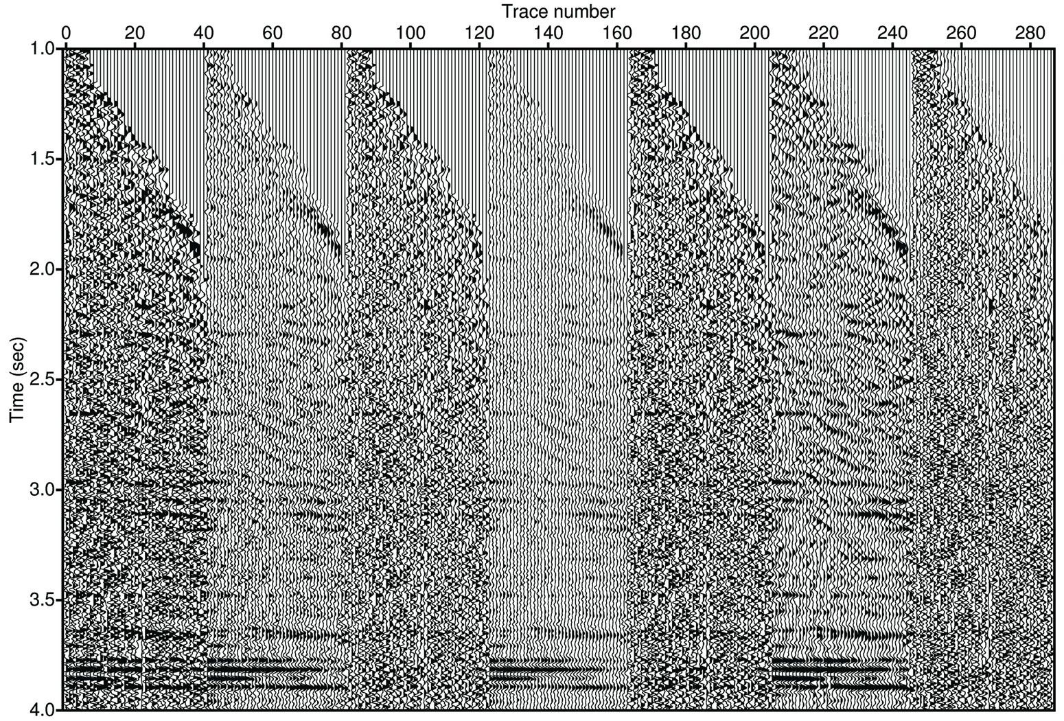
Figure 3 compares the two methods using a real dataset. The input data are not only contaminated by a large amount of random noise but also coherent noise (multiples and leftover ground roll). For the FX deconvolution, we tried different prewhitening coefficients to find an optimal solution. As the results show, the predicted data are either too noisy or too clean. If the prewhitening is increased signal leakage will also increase. In this example, the FX deconvolution cannot separate signal from noise. The result of the proposed method is better than conventional FX deconvolution at preserving the coherent signal. However, as shown in Figure 3, the new algorithm does little to the coherent noise. This is reasonable since the coherent noise is also locally linear, and it can pass the FX prediction filter.

Conclusions

We have proposed a new multi-channel noise reduction algorithm using TX domain deconvolution and FX domain prediction filtering. The prediction filters are computed from the data, saved for all frequencies, and used as a preconditioner for a multichannel deconvolution inverse problem. The method is not sensitive to wavelet errors when it is applied for noise reduction. Our tests show that the proposed method can be used as alternative to FX deconvolution to process, for instance, AVO gathers.

We have also used the method to enhance resolution of seismic records. In this case, precise knowledge of the wavelet is needed, as it is often the case with methods for resolution enhancement.