Beyond Isotropy – Part I: A Prestack Perspective

The seismic response is composed of two parts: the traveltime of a signal from the surface to and from a reflector and the amplitude of the reflection. Of interest here is the amplitude of the reflection, which is primarily a function of material properties at a given geological interface; specifically the density, compresional and shear velocities of the two layers that make up the interface. Reflection amplitude, is also a function of angle of incidence, and this is described by the Zoeppritz equations. These equations describe the incident amplitude becoming partioned at an interface into compressional and shear components. Approximations to the Zoeppritz equations have been made to simplify the understanding of the offset dependent reflection amplitude and allow for estimation of the interface constrast. One such approximation by Fatti et al. (1994), which will be discussed in greater detail, is commonly used for such purposes. Inverting the interface contrast, or reflectivities, allows for a rock properties perspective of the subsurface and interpretations of lithology, porosity and fluid type using seismic data.

Extending the same exercise to anisotropic media has become more important in recent years, whether it be to account for lamintated shales or an oriented set of vertical fractures. Determining the expected seismic signature of anisotropic rocks, however, is not an intuitive exercise. As opposed to the isotropic case where a combination of increase or decrease in P and S impedances determine the AVO type, the anisotropic AVO signatures have additional parameters that must be accounted for. In fact, it has been shown that the isotropic Rutherford and Williams (1989) AVO types can superimposed on a Lambda-Mu-Rho (LMR) crossplot by Hoffe and Perez (2008). This two part discussion, tackles the ability to extend AVO to include anisotropy on an LMR crossplot with the goal of ascertaining the prestack offset and azimuth dependent seismic signature jointly with the rock properties that govern the reflection.

In Part 1, a closer look at understanding the prestack seismic reflection in two different anistoropic settings is investigated. A simple diagram is presented that enables an intuitive grasp on the controlling factors of anistoropic reflections. The subsequent Part 2 will look at the ramifications on an LMR crossplot.

Isotropic Review

Before jumping into anisotropic relations, a quick reivew of isotropic AVO is provided. Consider the two-term isotropic approximation to the Zoeppritz equation, by Fatti et al. (1994)

where Ip is P-impedance, Is is S-impedance, Vp is compressional- wave velocity and Vs is the shear-wave velocity. The “bar” term indicates averaged quantities of the two layers, while D represents the difference between the second and first layer. Equation 1 can be divided into two parts: a zero offset component and an angle dependent component. To determine when this expression would have zero gradient, the angle dependent terms are set to equal zero.

Making the small angle approximation that tan2q ~ sin2q�� yields

Equation 3b gives the condition over which the angle dependent terms will have no impact on the measured amplitude. This equation is best represented by solving for shear reflectivity as a function of compressional reflectivity

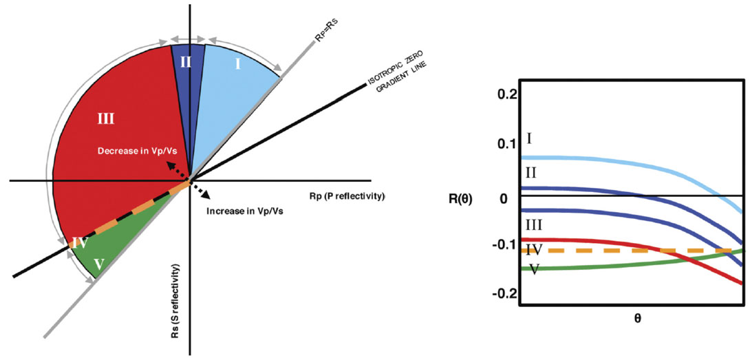
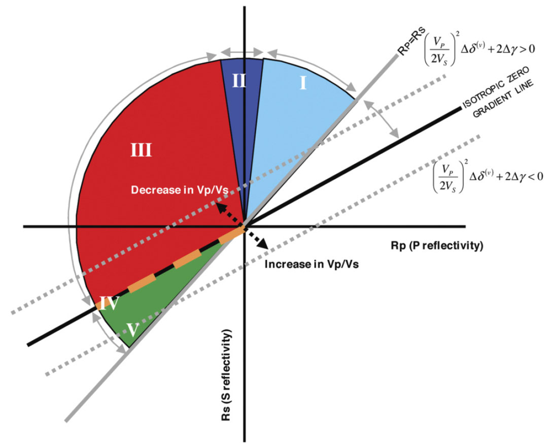
Equation 4 defines the zero-gradient line where if shear reflectivity is one-eighth the squared Vp/Vs ratio of compressional reflectivity there would be no angle dependent variations in amplitude. Crossplotting S reflectivity versus P reflectivity, (hereafter, Rp will refer to P-reflectivity and Rs, the S-reflectivity) allows for a visual display of all prestack seismic reflections, as described by the two-term Fatti et al. (1994) approximation.

In Figure 1 the coloured P and S reflectivity zones, referred to as the AVO reflectivity semi-circle, represent the normal AVO types as defined by Rutherford and Williams (1989) and are characterized by decreases in the Vp/Vs ratio. The two lines of importance on this crossplot are the Rp=Rs and the Rp=2Rs lines. The grey Rp=Rs line, represents the boundary separating Vp/Vs increases from Vp/Vs decreases. The black line is the Rp=2Rs line which in this case, assuming Vp/Vs=2, respresents the zero gradient line in accordance with equation 4. This line separates negative gradients from positive gradients. It follows that the larger the normal distance from a reflectivity pair (Rp, Rs) to the zero-gradient line, the larger the expected gradient. Note that most AVO types have negative gradients. The exception is Type 5, which has a positive gradient yet represents a decrease in Vp/Vs ratio across an interface. The AVO circle describes all possible prestack seismic reflections as a combination of Rp, Rs and Vp/Vs ratio as approximated by Fatti et al. (1994) two-term equation. The non-coloured portion of the AVO circle corresponds to non-reservoir AVO responses, most of which have positive gradients and increases in Vp/Vs ratios.

Anisotropic Extension

A similar procedure can be followed for any anisotropic expression. Below, the zero-gradient lines for Ruger’s (1997) three-term vertical transverse isotropy (VTI) and horizontal transverse isotropy (HTI) expressions are computed. The VTI angle dependent amplitude expression given by Ruger is

where Z is P-impedance and G is the shear modulus ρVs². The anisotropic terms are ε and δ as defined by Thomsen (1986) as

VTI media has a vertical axis of symmetry and can be used to model flat lying shales, oriented horizontal cracks, or thin beds of isotropic layers (Thomsen, 1986) As will be shown shortly, the parameters of particular interest are the δ and γ terms. Schematically, they are represented by portraying individual stiffness components shown in Figure 2.

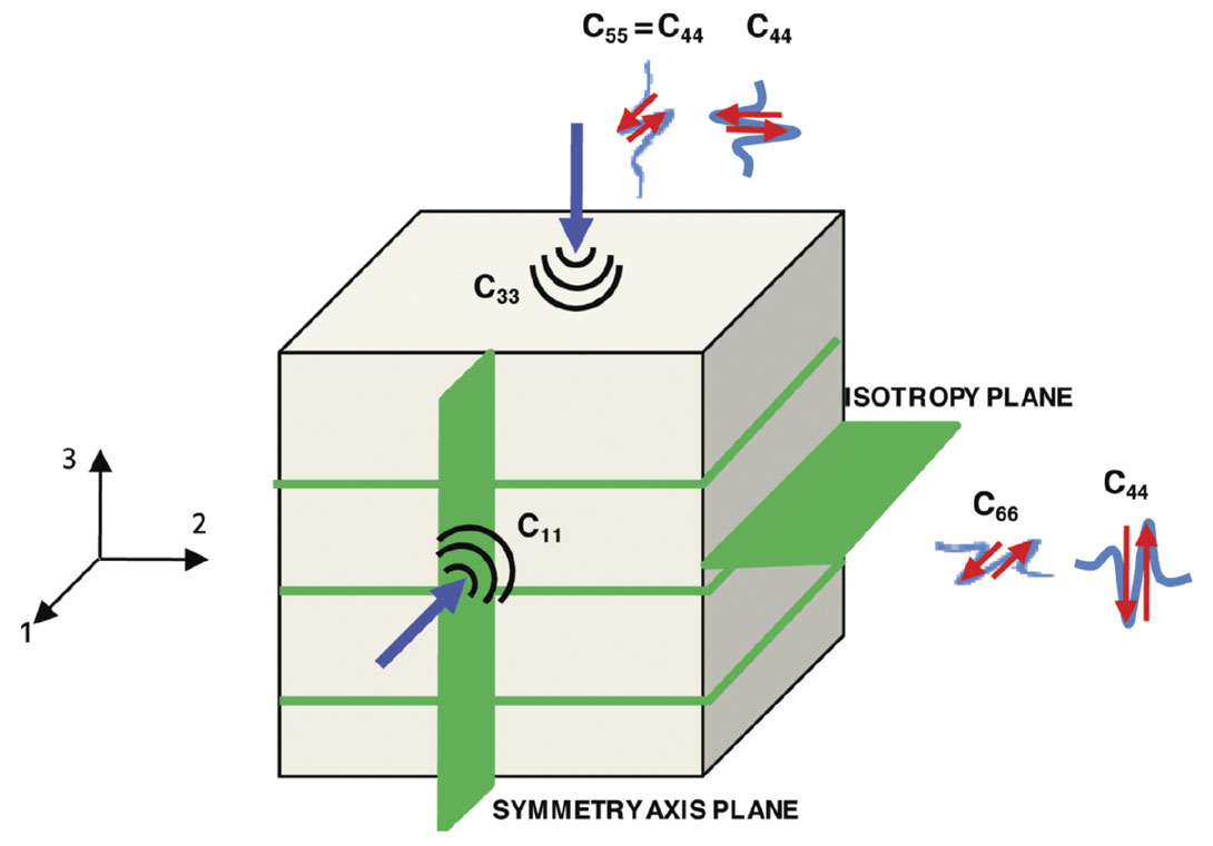
Note that ε and γ are the ratios of the fast and slow compressional and shear velocities, (V_fast-V_slow) / V_slow, respectively. The δ term is what controls the near vertical anisotropy (Thomsen, 1986). It contains the C₁₃ stiffness coefficient, which relates stress in the x directions to strains in the z direction, in combination with vertical stress-strain coefficient, C₃₃, and the slow/vertical (perpendicular to bedding) shear wave coefficient. The δ term, is possibly best understood as the scaled difference of compressional velocity at 0, π/4 and π/2, specfically given by (Thomsen, 1986),

Computing the zero-gradient line for VTI symmetry is achieved by equating the angle dependent terms to zero, making the small angle approximation and neglecting the quartic angle dependent terms in equation 5, which results in

This equation has a similar form to that of the isotropic two-term equation except for the additional d term. The HTI expression is given by

Ruger’s HTI expression does not use the γ^(V) term. However, for completeness, the anisotropic terms are ε^(V), δ^(V) and γ^(V) defined by Ruger (1997) specific to HTI media are shown below

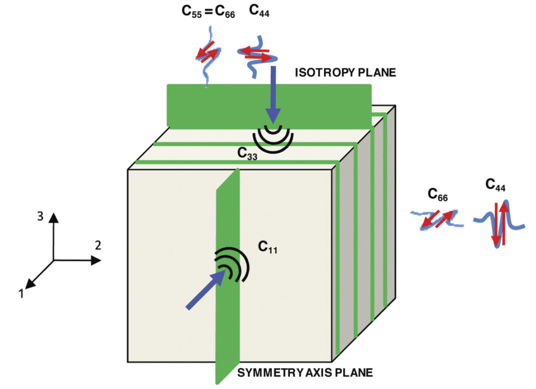
HTI media has a horizontal axis of symmetry and is used to represent a set of oriented vertical fractures. To maintain the (V_fast-V_slow) / V_slow of these expressions, the order of stiffness indeces must be reversed, relative to the VTI case. Note that the same C₁₃ stiffness coefficient in combination with vertical Pwave velocity and the slow shear wave velocity coefficient in δ^(V) obscures the parameters physical meaning. The anisotropic parameters in VTI and HTI media are related in the following way

and assuming weak anisotropy,

Schematically, the anisotropic parameter ε^(V), δ^(V) and γ^(V) terms are represented by the stiffness coefficients in figure 3.

As with the VTI expression, the quartic angle dependent terms are neglected. In addition, because of the existence of azimuthally dependent components, equation 9 is computed in two directions: parallel to fracture (π/2), and cross-fracture (0). The parallel to fracture direction results in

which is essentially a scaled version of the Fatti et al. (1994) isotropic expression. The cross-fracture direction reduces to

Recasting equations (8) and (14) to solve for shear reflectivity results in the following expressions for VTI and HTI media, respectively:

These are equivalent to the B^ani expressions of Bakulin et al. (2000). The focus of the following discussion will be primarily on HTI media. A similar argument not only follows for Ruger’s VTI expression but also different angle and azimuthally varying amplitude expressions for HTI and VTI media.

In Figure 4 the zero-gradient line on a P and S reflectivity (Rp-Rs) crossplot provides inisght on how changing the media to VTI or HTI anisotropy will affect the seismic signature. In Ruger’s HTI expression,

as the compressional (P) and shear (S) reflectivity (Rp and Rs, respectively). The effects of the anisotropic terms can be assessed by considering their impact on the position of the zero-gradient line on an Rp-Rs crossplot. In the HTI case, the anisotropic terms, ¼(Vp/Vs)²Δδ^(V)+2Δγ , determine the y-axis intercept of the zerogradient line.

This implies that a given P and S reflectivity combination in isotropic media may produce a Type 3 reflection but with appropriate combination of anisotropic parameters, the seismic signature could exhibit a Type four– no gradient – reponse. (Note: The VTI case would have equation (15a) defining the new zero gradient line.) Again, the gradient term is expected to be larger when the the normal distance from reflectivity pair to the zerogradient line increases.

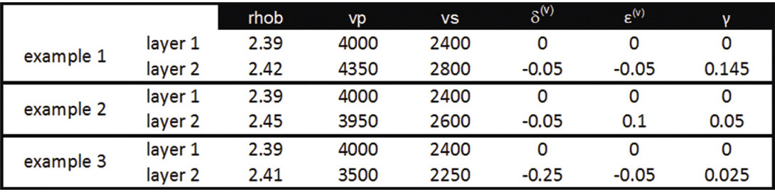
Consider the three following reflectivity pairs (NOTE: In the following models, the full three-term expression is used to create the synthetic AVO responses.):

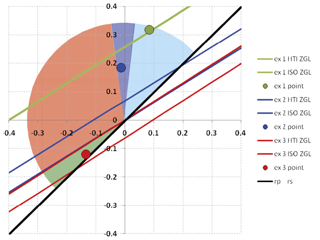
The Rp-Rs crossplot representation and aziumthally dependent AVO responses for these three examples are seen in figure 5 and 6 respecitvely. In example 1, the reflectivity pair (positive P and S reflectivity) would exhibit a Type 1 response in the parallel to fracture, π/2, orientation. This would also be the response if both layers were isotropic. In the cross fracture direction, the combination of anisotropic parameters yields positive anisotropy (¼(Vp/Vs)²Δδ^(V)+2Δγ > 0) which superimposes the zero-gradient line on the Rp-Rs pair for example 1. Thus the response would be of Type 4, a zero-gradient response. This example shows the small angle approximation used as at larger angles a slight positive gradient is observed.

In example 2, the parallel to fracture orientation, would exhibit a Type 2 AVO response (very small P-reflectivity, positive S-reflectivity). The example has positive anisotropy (¼(Vp/Vs)²Δδ^(V)+2Δγ > 0) and thus as the azimuth moves towards the cross fracture orientation the AVO response will move towards a smaller gradient Type 2 response.

The third example exhibits a slight Type 5 response, in the parallel to fracture orientation (negative P and S reflectivity). For the cross fracture direction however, the negative anisotropic terms (¼(Vp/Vs)²Δδ^(V)+2Δγ < 0) have moved the zero-gradient line to the other side of the reflectivity pair, resulting in a change of gradient polarity. As expected, the observed AVO type in the cross fracture direction is of Type 3. A similar argument follows for VTI media.

Conclusion

This first of two parts investigates the controlling parameters for angle and azimuthally varying amplitude in anisotropic meida. Relating the anisotropic AVO types to the isotropic case through the zero-gradient line shows that for VTI media, the δ parameter affects the angle dependent amplitudes, while in HTI media, δ^(V) and γ both play a role in varying amplitudes with angle and azimuth. Crossplotting P and S reflectivities in conjuction with with the zero-gradient line facilatates a quick determinination of AVO type and the expected variation for a given set of anisotropic setting and parameters.