Perusing my recent articles, I realized I’ve been touching on some rather somber topics lately, such as mental illness, psychopathy, prion disease, Nazi death camps, etc. So this month I decided to lighten things up and cover some cheerful examples of how science can be applied in day-to-day ways. Astute readers will see through this explanation, and quickly assume I am running short of topics. It may be a bit of that, but the truth probably lies somewhere in between – it’s the dog days of winter and dredging up the energy to research and properly cover a complex topic just seems so daunting compared to watching TV or doing crosswords. I’ll be off to a beach vacation in a couple of weeks, and I expect that will re-energize me for next month’s article on corals.
Alcohol and Winter
You’re not Canadian if you haven’t been faced with this dilemma – “Is it too cold to leave my beer or wine in the car overnight?” Well this is the sort of situation where science can be put to a practical use for a change. I mean really, is my quality of life going to be affected if they prove the existence of the Higgs boson? But if I can confidently leave my drinks in the car to chill before tomorrow’s trip to my imaginary multi-million dollar ski chalet at Blue “Mountain”, and save myself the trouble of lugging them to the refrigerator and back, then I’m a happy man. We all know that alcohol has a lower freezing point, so beer and wine can be stored at temperatures lower than 0 °C without freezing, but how much lower?
It turns out to be not entirely straightforward, because alcoholic beverages are a mix of water, alcohol, and other components. As the temperature drops below freezing, the water freezes but the alcohol doesn’t, creating a form of slush. As more and more of the water freezes, the remaining liquid has a higher and higher alcohol content which lowers its freezing point. Incidentally, this is a poor man’s alternative to distillation, and is also used at a commercial level – that is how ice beers achieve a higher alcohol content. This has been done for centuries; for example, in Germany there is a longstanding tradition of beers known as Eisbock. The beer is chilled when it is close to fully fermented, and ice crystals form. The remaining liquid is drawn off, creating a beer that is up to 10% alcohol, twice the strength of regular beer. I intend to try this with cider, maybe this weekend. But I digress…
Let’s assume our drinks are just water and alcohol – that will allow us to get ballpark estimates, which should be good enough for our purposes. What we’re going to use is the chemistry concept of freezing point depression, which applies to any situation where there is a solution formed by the mix of a solvent (water in this case) and a solute (alcohol in this case), and the freezing point is required. The formula is:
ΔTf = Tf (pure solvent) – Tf (solution)
ΔTf = Kfm
where:
ΔTf is the freezing point depression, and Tf denotes the temperature at which freezing occurs,
Kf , the cryoscopic constant is solvent dependent, (for water Kf = 1.853 K*kg/mol);
m is the molality (moles solute particles per kg of solution).
Let’s try it out for a New Zealand Sauvignon Blanc with 12% alcohol content, and assume we have 1000g of wine – that means 120g of ethyl alcohol (C2H6O) and 880g of water (H2O).
To determine the molality, first we need to calculate the number of moles of C2H6O in the wine. C2H6O has a molar mass of 46.07g/mol, so,
Moles of C2H6O in the bottle of wine
= (Mass C2H6O) / (Molecular Weight C2H6O)
= (120g C2H6O) / (46.07g/mol C2H6O)
= 2.60 mol C2H6O
Molality of wine = (Moles Solute) / (Mass Solvent)
= (2.60 mol CH3OH) / (0.88kg H2O) = 2.96m
With that done, we can now plug the result into the freezing point depression equation.
ΔTf = Kfm
= (1.86m/°C)*(2.96m)
= 5.5 °C
ΔTf = Tf (pure solvent) –Tf(solution)
Tf (solution) = Tf (pure solvent) – ΔTf
Tf (solution) = 0 °C – 5.5 °C = – 5.5 °C
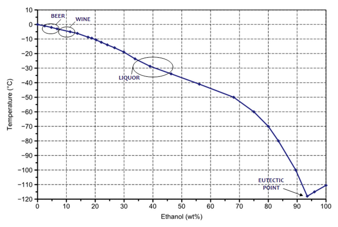
So we’d expect our wine to freeze at -5.5 °C. Going through the same exercise for hard liquor (40% alcohol) and beer (5% alcohol) gives freezing points of -26.9 °C and -0.2 °C respectively. The presence of other substances in these drinks (sugar, sulphides, etc.) pulls the freezing point down a bit more, and the slushy effect I mentioned above does as well. The handy chart in Figure 1 shows the freezing point curve of a water / alcohol solution, and I’ve superimposed freezing point estimates, which are beer at ~-2.5 °C, wine ~-5.0 °C, and liquor ~-30.0 °C. The labels on bottles show the percent alcohol volume, whereas the equations and the graph are based on percent by mass, so that explains the difference in numbers somewhat.
The eutectic point is interesting as applied to another winter topic – the use of salt to prevent ice on roads and sidewalks. In Toronto they dump mountains of the stuff everywhere. I’m aghast and can only speculate what it’s doing to the environment. The eutectic point represents the temperature at the lowest melting point for a substance made up of two or more components. Adding salt to water lowers the melting point, which is desired to prevent slippery conditions, but the eutectic point for that mix is -18.0 °C. In Calgary, where winter temperatures are often lower than that, sand and gravel become the preferred method for dealing with ice. In Toronto where winter temperatures aren’t as cold, salt is used extensively, and the lower range is extended a bit by the additional use of liquid antifreeze agents.
Thunderstorms
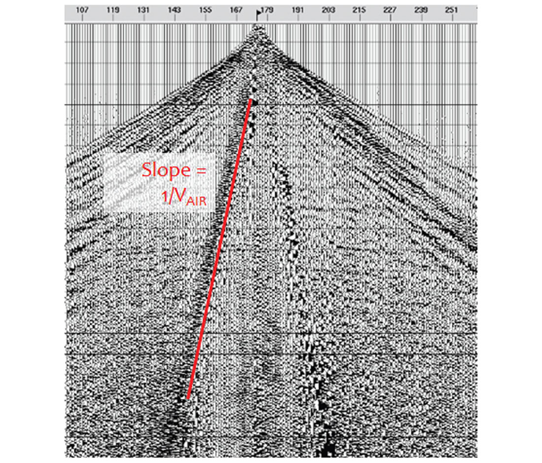
It borders on insulting to present this topic to a readership made up largely of seismologists, who should be familiar with the velocity of sound in air. But let’s make the reasonable assumption that unless a person is exposed to a scientific concept or fact on a routine basis, they will forget it as soon as the last exam on the subject is handed in. Seismic processors are familiar with air blast noise trains on raw shot records (Fig. 2). These are generally caused by hissing noises given off by the hydraulic systems in Vibroseis trucks. The sound waves travel through the air and are picked up by the geophones. The slope of these noise trains gives the known velocity of sound waves in air, which is 343.2 m/sec in dry air at 20 °C. Given that, it’s easy to estimate the proximity of a lightning strike, if you can estimate the time between seeing the flash of lightning and hearing the thunder. Why this is of any use is beyond me, but as a boy I was very impressed by people who could do it. I think a good rule of thumb would be to say that each 3 seconds of time represents about 1 km. For the time estimate, I recommend using the “Mississippi one, Mississippi two, …” count method.
Estimating Heights
When I was a Cub Scout, I remember getting a badge for learning some impossibly complicated way of estimating the height of an object, like a tree or cliff. As I recall it involved estimating angles, which right there makes it unreliable in my mind. Since then I have learned a much easier way of doing this.
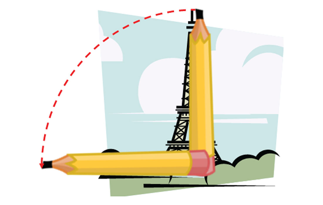
First, find something like a pencil or straight stick. Hold it vertically upright in your hand with your arm straight ahead of you. Close one eye and squint in a manly fashion (or womanly as the case may be) and line up the top of the feature being measured with the top of the pencil. Slide your thumb so it lines up with the bottom of the feature. Now rotate the pencil 90 ° holding your thumb in place so that the pencil is horizontal and your thumb is still at the base of the object. Make a mental note of some object that lines up exactly with the tip of the pencil. Now simply walk over to the base of the object and pace off the distance from there to the object you identified – this distance will reasonably represent the height of the object. This is just simple geometry – you’ve scribed a simple quarter circle with your thumb as its axis, and the radius is the height of the object. I’ve tried to depict this method in a picture (Fig. 3), if you can imagine holding the pencil up so it lines up with the Eiffel Tower.
The key to this technique is to accurately pace off the distance between the two points you’ve identified in your mind. To achieve this you’ll have to know what your typical stride length is, something that is second nature to golfers, who routinely pace off the distance between fixed distance markers and where their ball lies, in order to estimate the distance to the hole.
A quick and dirty alternative to this approach is to keep splitting the unknown object’s height in half (visually) until you can compare your divided height with an object at the base of known height. Each time you split the height in half means you have to multiply your known object height by another factor of 2 to get your estimate. In other words, you multiply your known object’s height by 2 raised to the power of the times you’ve divided the unknown object’s height in half. For example, the Eiffel Tower is 324 m high (but you don’t know that). If you visually divide it in half 8 times, you’re down to 1.27 m (324 / 162 / 81 / 40.5 / 20.25 / 10.125 / 5.06 / 2.53 / 1.27). Now say Toulouse Lautrec is standing at the bottom and your Eiffel Tower-divided-by-8 height visually seems about the same height as him, and you happen to know his height is about 1.3 m. Just take that 1.3 m and multiply it by 28.
H = 1.3 * 28 = 1.3 * 256 = 333 m
Going the other way, it’s common to want to know how far down something is, like the bottom of a well, or the distance from the top of a cliff to the bottom. The good thing about these situations is that you’re in control of the experiment, which involves dropping an object and timing how long it takes to get to the bottom, plus nowadays everyone has a timer and a calculator on their phone. This is all grade 10 physics, so in other words, impossibly difficult for most of us without a refresher. The velocity of a body under constant acceleration, starting from rest, at time t, you’ll vaguely remember is given by,
V = a * t
Where a is the constant force of acceleration. On earth, at sea level, with no air resistance, this value is 9.80665 m/s2. Integrating the formula for velocity gives the corresponding formula for distance travelled, for the same body under constant acceleration, starting from rest.
D = ½ a * t2
This is the equation we need to use, and given it’s a crude experiment designed to come up with an estimate only, we’ll ignore the effects of air resistance, and round the 9.80665 to 10. We can minimize the air resistance error by choosing an object with low air resistance, such as a round stone or maybe a jellybean (versus, say, a piece of chewed gum). If we’re going to use sound as the method for determining the time when the object hits bottom (versus a visual of the angry man with gum on his head looking up), then there is an error there as well. You now know sound travels ~343 m/s, but to save you the trouble of coming up with a recursive ballpark correction, I’ve put together the following little chart of time corrections to account for the time it takes for the sound to get back to you – simply locate your recorded time in the “In air” time column, roughly interpolate the “Correction”, then subtract this correction from your recorded time.
| Time (seconds) | |||
|---|---|---|---|
| Height (m) | In vacuum | In air | Correction |
| 50 | 3.19 | 3.34 | 0.15 |
| 100 | 4.52 | 4.81 | 0.29 |
| 200 | 6.39 | 6.97 | 0.58 |
| 300 | 7.82 | 8.70 | 0.87 |
| 400 | 9.03 | 10.20 | 1.17 |
| 500 | 10.10 | 1156 | 1.46 |
| 600 | 11.06 | 12.81 | 1.75 |
| 700 | 11.95 | 13.99 | 2.04 |
| 800 | 12.77 | 15.11 | 2.33 |
| 900 | 13.55 | 16.17 | 2.62 |
| 1000 | 14.28 | 17.20 | 2.92 |
So all that’s required is to time the dropping object, subtract the correction if using sound, then square the time and multiply by 5 ( ½ * 10) and you’ve got your estimate. For example, the Eiffel Tower observation deck is 276 m above ground (but we don’t know that). We drop our piece of gum, and the shouts of l’homme en colère reach us 8.3 seconds later. Glancing at the chart we apply a rough correction of 0.8 seconds, giving a corrected time of 7.5 seconds. Our crude estimate for height above ground is given by,
H = ½ * 10 * 7.52 = 281 m
Jellybeans
Most people are subjected to a jellybean guessing contest at some point in life, or something similar, especially if they have children. Usually there’s a jar of jellybeans, and the person who comes closest to guessing the actual number of jellybeans in the jar wins the jellybeans. How exciting is that?! Now I will ask readers to make a large leap of faith, which is to assume there actually exist among us some who would want the jellybeans badly enough to prepare ahead of time a method to more accurately estimate jellybean numbers.
What is required to win the jellybeans actually involves three estimates – the volume of the container, the volume of an average jellybean, and the ratio of pore space (air) to matrix (jellybean).
To estimate the jar size, it helps to realize that most jars and containers come in standard sizes. However, given the use of both metric and imperial sizes here in Canada, this is a dangerous game, and as a scientist you should be self-reliant – use those simple geometrical formulae you thought you’d never need! As you’ll recall, the volume of a cylinder is given by the product of its height and the area of its base, so
Vcyl = h * (πr2)
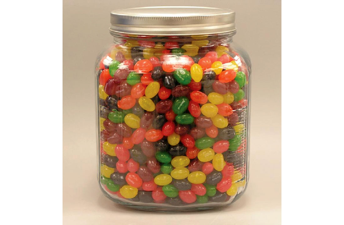
That should suffice to give an estimate of the jar’s volume, but remember not to mix up radius and diameter! Reduce your estimate appropriately if it has a curved top and bottom as in Figure 4. If it’s a rectangle, then volume is even easier,
Vrect = h * w * d
And for a sphere,
Vsph = 4/3 * (πr3)
To estimate the volume of a jellybean, it can be approximated by a cylinder as well. Lastly, what percentage of the jar’s volume is made up of air? This is similar to approximating pore space percentage from a thin section, an area in which geologists may have an advantage. What I can tell you is that I have researched this extensively, and the jellybean geology experts agree that 20% is a very good number to use. So to put it all together, calculate the volume of the jar, multiply that by 0.8, and then divide that by the volume you’ve calculated for one jellybean. That will give you a very good estimate of the number of jellybeans in the jar. Good luck!
Eggs – Soft or Hard?
There are a couple of simple science-based tests to determine if an egg is raw or cooked. To be honest, I have totally forgotten all the physics surrounding rotating bodies, bearing credence to my earlier assumption that most knowledge is quickly forgotten after university. And as per my earlier comment, I am in no mood to read up on the physics of rotating bodies of different rigidities. However, I am totally confident in the knowledge that a rigid rotating body will spin longer and faster than one of equal size and mass that is deformable. For example, a singles squash ball, which is very squishy and deformable, loses its spin very quickly, whereas a doubles squash ball, which is hard, spins a lot and retains that spin even after bouncing off two or three walls, with baffling effect. With the soft squash ball, most of the energy of the spin is converted to deformation, and this acts as a damper on the spin.
A soft egg is a deformable body with a rigid shell, whereas a hard-boiled egg is hard throughout. This difference is manifested in the ways the two kinds of egg spin. If you have an egg of unknown hardness, place it on a flat hard surface like a table, and give it a spin. If it spins fast and smooth, it’s likely hard-boiled; if it wobbles as it spins and slows down quickly, it’s likely raw. If it falls somewhere in between, it’s likely soft-boiled. Further, if you stop the spinning egg by gently placing enough pressure with a finger from above, a hard-boiled egg will stay stopped, whereas a soft egg will actually start to spin slightly again. This is because the soft insides have not stopped moving, and this internal movement causes the egg to start spinning a bit again. If you take a cooking egg out of the boiling water, a hard-boiled egg will dry off very quickly (~10 seconds), whereas a soft-boiled one will stay wet for a while longer (~20 seconds). This is because the hard-boiled egg holds greater residual heat.
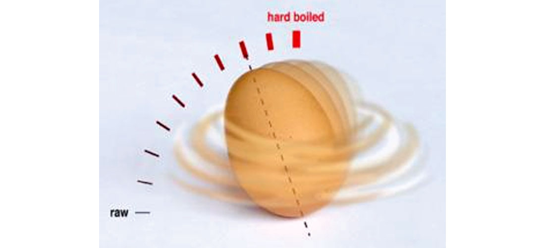
I found one fun reference to egg spinning (RedStateEclectic, 2010) which contains a poem, a picture, and a video clip, describing how a hard-boiled egg will end up spinning on one of its ends. Start the egg spinning horizontally at a rate of at least around 10 rotations per second. If it is hard-boiled it will quite quickly stand up on end and spin faster, just the way figure skaters spin faster when they pull their arms and legs in. This probably has something to do with polar moment of inertia or some equally baffling concept, so I say let’s just finish off with this spinning egg poem, and move on to next month!
Place a hard-boiled egg on a table,
And spin it as fast as you’re able;
It will stand on one end
With vectorial blend Of precession and spin that’s quite stable.


Share This Column