Expert Answers

Question 1

In the 1970s and the early 1980s, geophysicists working in offshore areas relied on spotting anomalies, where not being so knowledgeable about structural geology was not so much of a problem. In other words the attitude was to pick up these anomalies without going into why they were there. And this worked e.g. in the Gulf of Mexico and other areas. Later they started using AVO to confirm such anomalies. When you talk about ‘deeper’ exploration, the rocks become denser and so the variable densities or porosities you are looking for are not there, i.e. DHI effects decrease drastically with depth. Besides, the AVO response in these areas may or may not conform to the structures present. What strategy do you adopt in such cases for detecting anomalies?

Answer

The first thing to make clear is that we wouldn’t now drill prospects based only on DHI’s. We have long recognised that we can be fooled – by lithology changes masquerading as amplitude conformance, by diagenetic changes looking like flatspots, by clean wet sands appearing as bright as nearby hydrocarbon sands (and having large AVO anomalies) and of course by residual gas. So now, when we look at seismic anomalies, we do worry about “why they are there”. We need to understand how the petroleum got to the reservoir, to understand the trapping geometry and the nature of the reservoir as well as the seismic response. We must reconcile “bottom up” prospecting with “top down”. We must take account of our understanding of the petroleum system, the nature and location of the source rocks and the migration pathways together with analysis of direct hydrocarbon indicators. This becomes increasingly important the deeper we go.

Another important thing to say about DHI’s is that using amplitude alone, either relative or an estimate of absolute impedance, is not enough. We need some evidence of a fluid contact; either a change of amplitude conforming to structure or a flat spot or both. All the edges of the DHI must correspond to trap edges so DHI’s must be interpreted in a way that is consistent with an understanding of the structural geology and the stratigraphy. No more “blobs floating in space”.

Optimum seismic data quality is of course paramount so due consideration must be given to appropriate acquisition, noise reduction and imaging strategy. For DHI analysis extra consideration must also be given to correct design of the final products. This requires an understanding of the local rock properties. There are a number of different forms of rock property analysis. One is to use the impedance equivalent of intercept/ gradient space, referred to acoustic impedance/gradient impedance or AIGI. By crossplotting the reservoir/ non- reservoir data from analogue wells or trend curves in AIGI space we can determine the optimum rotation angle to maximise sensitivity to fluid changes as well as the percentage impedance change that a given fluid change will cause. However, determining a detectability threshold is very difficult and will depend on many factors such as the extent of the fluid contact, the signal to noise of the seismic, the influence of the overburden, reservoir heterogeneity etc. all of which may be hard to estimate.

A constant angle stack should be produced corresponding to the projection in AIGI space that shows greatest sensitivity to fluid change. In practice, angles from rock property analysis will differ from the calculated seismic angle due to anisotropy and our inability to correctly scale the data so it may be necessary to scan through a range of coordinate rotations and select the best. Coordinate rotations corresponding to incidence angles beyond the seismic spread will have decreasing signal to noise so it may be better to compromise on a lower angle. Pragmatically, a far angle stack is usually a pretty good option.

If the shale or non-reservoir points lie away from the fluid line on the AIGI crossplot then it should be possible to construct a data volume which is insensitive to fluid changes but sensitive to lithology contrasts. If the fluid volume shows conformance but the lithology volume does not this effectively removes the risk of a lithology edge being misinterpreted as a contact and greatly adds to our confidence in interpreting the conformance as a fluid contact.

Another process that is finding widespread application is coloured inversion. This shapes the spectrum of the seismic data to be as close as possible to that of an impedance log within the limits of the seismic. Invariably the spectrum can be effectively approximated as a power law function, linear on a dB/log freq plot and decreasing with frequency. Coloured inversion (CI) ensures that the seismic wavelet has a flat-topped spectrum and hence provides optimum resolution. The analogous process in the reflectivity domain is “blueing” which shapes the seismic trace to the equivalent linear blue shape and so also will have the same flat-topped wavelet. The advantage of the impedance domain is that the frequencies having the highest signal to noise are more prominent thereby increasing the overall signal to noise of the data while retaining optimum resolution.

Detailed, “surgical” interpretation of the prospect should now be carried out, carefully picking every loop over an area sufficient to put the prospect into context. Picking is best done by tracking zero crossings on the CI data, which allows attributes to be extracted between the top and base picks. If average amplitude, or similar, is calculated then a detuning algorithm can also be applied to remove the effects on amplitude of variable thickness.

Finally the horizons need to be accurately depth converted and depth contours displayed superimposed on the attribute maps to analyse for conformance. This should be done independently for each horizon; it is not good enough to just use contours from a regional horizon.

So in summary, integration is the key. Reconcile the observed seismic response with an understanding of local rock properties, the structural geology (and the evolution of the structure), knowledge of the reservoir and the petroleum system. By doing all this we can successfully push deeper our application of DHI analysis.

Pat Connolly
BP, UK

Question 2

Elastic properties of materials such as shale and chalk are anisotropic, still AVO analysis are routinely carried out assuming the media to be homogeneous and isotropic. How significant are the effects of anisotropy on reflectivity and how can we go about accounting for them in the interest of more accurate and realistic AVO interpretation?

Answer

To be meaningful, all seismic amplitude analyses require that the pre-stack data be accurately positioned both laterally and vertically (in time or depth). This necessitates the use of imaging and processing flows appropriate to the geology of the area and the seismic acquisition geometry. A discussion of these flows is beyond the scope of this short article, where I assume that the data has been migrated and processed optimally, such that the waveforms in the gathers are properly positioned, “clean” and adequately balanced for amplitude and frequency, without migration artifacts being imposed.

In general, it is appropriate to make a distinction between AVO analyses in an <1> Exploration world, where new reservoirs and seals are being tested for the first time, from AVO analyses performed in <2> an Appraisal & Development mode, where copious amounts of well data add to the seismic interpretation process.

<1> Exploration-Reconnaissance AVO. “Recon” AVO suffers from the lack of adequate well control, and hence is not truly quantitative. Due to insufficient information, it is often not properly calibrated to rock properties or seismic lithology-fluid modeling studies. As such, the effects of anisotropy are often ignored at this stage. Numerous unknowns typically do not allow for non-unique low-risk interpretations of pre-stack seismic amplitudes, but the value of the technique has nevertheless been recognized by industry, as most prospects undergo amplitude and AVO studies of some sort, prior to being ranked and moving into a portfolio of possible drilling candidates.

Recon AVO is a powerful tool, which when integrated with other techniques, contributes to the drilling decision process, regardless of whether anisotropy is taken into account. It is interesting to note that Recon AVO has been particularly successful in certain types of geological environments and hydrocarbon provinces, notably in deltaic and turbiditic sequences of basins with relatively simple tectonic histories (ie: Tertiary basins of Gulf of Mexico, Nile delta, West Africa, Offshore Brazil, as well as older basins, such as the North sea), where type III AVO (Rutherford and Williams, 1989) is the rule.

In Exploration/Recon AVO, a robust 2-term AVO approximation (ie, Shuey, 1985) is often used, and Intercept and Gradient techniques, or other equivalent two-parameter cross-plotting methods, have been applied successfully.

<2> Appraisal-Development AVO. Seismic amplitude and AVO analyses, when used for Appraisal purposes, have the objectives of assessing the extent and quality of a reservoir system (defined as the interaction of a reservoir and its seal) and the type or amount of reservoir fluids (hydrocarbon versus brine, in-situ PVT, and if at all possible, hydrocarbon saturation).

The key to Appraisal AVO is to infer “semi”-quantitative interpretations from seismic signatures, after local calibration to wells and the construction of rock property models. The objective is to go beyond qualitative interpretation and achieve an understanding of subtle changes in the seismic signal in terms of geology, fluids or in-situ conditions. This requires incorporating anisotropic effects and often involves “higher term” AVO analysis, which may also lead to extracting density information.

As a consequence, in Appraisal AVO it is often necessary to go beyond cross-plotting techniques and use a three-term AVO equation. One must rely on pre-stack inversion methods, which yield Vp, Vs and sometimes density, where the data quality permits it. If cutting-edge techniques are used (shear wave source for example), there is also hope to invert for fluid saturation from the ratio of P-to-SH wave reflections (Wright, 1986).

Anisotropy can have a significant effect on seismic amplitudes. This has been documented extensively, both in the laboratory as well as mathematically. Analytic expressions were derived for elastic Vertical Transverse Isotropy –VTI- (Thomsen, 1986, Banik, 1987, Alkhalifa and Tsankin, 1995), and the effects of anelasticity (or attenuation, Q) in VTI media were discussed (Samec and Blangy, 1992, Blangy, 1994). The elastic VTI expressions were extended to the case of Horizontal Transverse Isotropy -HTI- (Rueger, 1997) and to orthorhombic anisotropy (Tsvankin, 1997). As discussed by Thomsen (2002), anisotropy affects AVO in two ways:

• by modifying the coefficients (the slope and curvature) of the AVO equations. This “dynamic effect” depends upon anisotropic contrasts at the reflecting horizon.
• by modifying the angles of the AVO equation, converting from ray-angle (as produced by the migration algorithm) to wavefront angle. This “kinematic effect” depends upon anisotropy throughout the overburden.

VTI (also referred to as polar anisotropy) is typically encountered where layer-induced anisotropy is present and where structural dip is small. This often occurs in geological environments with an extensional structural style (rifts for example) and near the crest of structures. VTI requires the use of 5 parameters in addition to density, but this reduces to 4 parameters for a P-wave source. These are Vp, Vs, δ and ε (Thomsen’s parameters or one can also use Tsvankin’s parameter η=(ε−δ)/(1+2δ)). Most majors and/or service companies have developed technology to characterize VTI media. The biggest challenge no longer resides in deriving the appropriate equations for modeling/migration algorithms nor does it lie in the computing power required for the computations, but it is found in appropriately characterizing those key anisotropic parameters. At the root of the parameterization problem lies (1) an inherent uncertainty in the nonuniqueness of the solution (ie, “I can focus the energy equally well with an isotropic model”) and (2) the poor resolution of those anisotropic parameters.

Anisotropy is a function of scale. It needs to be estimated in the context of the scale of the dominant seismic wavelength with respect to the geological objects being traversed by seismic waves. While seismic methods currently allow for low resolution estimates of VTI parameters, predictions can be obtained at a finer scale through the use of well data (cores, logs, VSPs), coupled with calibrations to geological/petrophysical models and then upscaling to seismic wavelengths (Backus, 1962, Hornby et al, 1994). This is the subject of much on-going research. In general, the vertical or time-to-depth velocity (Vp0) is related to δ and the P-wave NMO velocity as in VNMO(0) = VNMO(0) = Vp0 1+ 2δ, but δ cannot be recovered from surface moveout information alone. It requires independent information, either from the moveout of S-waves or preferably from well data. The parameter η can be estimated from moveout information, ie through non-hyperbolic moveout.

Azimuthal anisotropy can occur where vertical fractures develop, which typically happens in compressive or strike-slip environments, where the minimal stress is vertical. A special case of limited interest is Horizontal Transverse Isotropy (HTI). Recent experiments at the core scale in the laboratory have documented that orthorhombic (azimuthal) anisotropy can be stress-induced (Sarkar et al, 2003). Parameterizing either HTI when in the presence of dip, or characterizing orthorhombic anisotropy, can require up to 9 parameters. This is not currently manageable in a production environment, nor do we know how to determine those parameters with confidence. However, we can “lump” these parameters together in the third term of the AVO equation, so there is hope for the future, as suggested by Thomsen (2002). Shen et al (2002) numerically investigated the effects of fractures (a typical situation in carbonates) on the main anisotropic parameters δ, ε and γ and concluded that P-wave azimuthal variation in AVO results from the complex interaction of fracture density, fluid content and seismic tuning to the reservoir thickness. Modern acquisition and processing efforts with Multi- Azimuth seismic and Ocean Bottom Seismic (OBS) will drive breakthrough advances in this area.

Anisotropic effects are particularly important when contrasts in Acoustic Impedance are small and significant changes in anisotropy exists across a seal/reservoir system. For siliclastic, this can happen at depths near the sand-shale cross-over (Neidell and Berry, 1989). It is the contrasts in anisotropy that lead to the departure in amplitudes from an isotropic reflection.

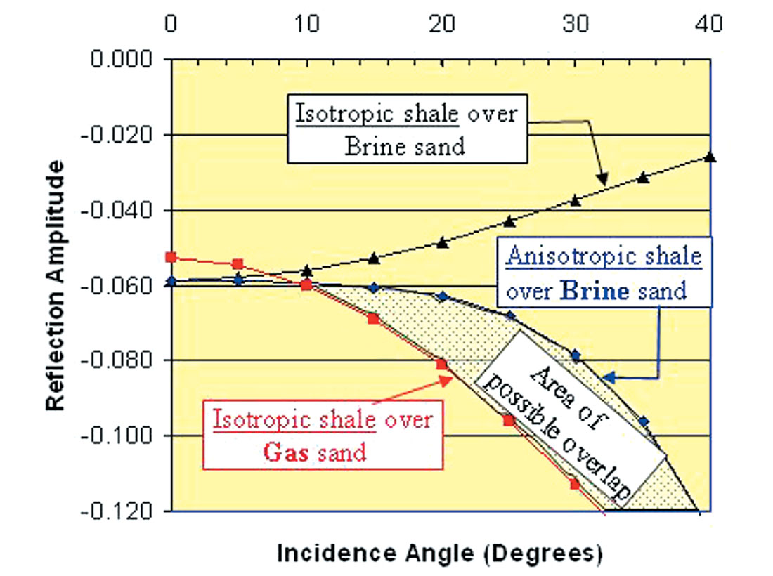
Anisotropic effects are more pronounced at larger angles of incidence (beyond ~20 degrees) where contributions from terms involving contrasts in δ and the difference in contrasts between δ and ε, modify the isotropic reflection. In general, it can be said that δ has a first order influence on AVO gradients, while ε dominates only at large angles of incidence. Ignoring anisotropy could lead an interpreter to make a costly mistake. For example, a brine sand overlain by an anisotropic shale could be mistaken for a gassy sand, should one fail to account for the anisotropy, as in the area of potential overlap shown in Figure 1.

<3> A VTI case study: Next, I present an example of Appraisal AVO, where the effects of anisotropy on pre-stack seismic amplitudes were quantified. I use a generic Gulf of Mexico deepwater example to preserve confidentiality. The sedimentary sequence is formed of siliclastics (sand and shales), which were deposited in a turbiditic environment (Miocene) capped by shallower deltaic and shoreface sediments (Pliocene, Holocene). The parameter δ was estimated from well data as the amount of seismic depth stretching was calibrated by a VSP. The parameter ε was obtained from moveout analysis and a migration scan was used to confirm that it lead to better focusing of the seismic energy.

Pre-stack gathers were modeled using well data and commercial software, for both the case of an isotropic shale (used as a reference, albeit unrealistic) and an anisotropic shale (Figure 2). The anisotropic parameters were determined as above and then approximated on a depth-continuous, sample-by-sample basis, using a shale model. The parameter δ varies from 0 to +/- 0.15, while ε ranges from 0 to 0.25, depending on the lithology. The top of the reservoir gives rise to a very weak reflection, but the base-of-reservoir reflection from the underlying shale is quite strong (the normal incidence Reflection Coefficient or RC=0.055) and exhibits an increase in Amplitude versus Offset (RC=0.125 at ~22,000 ft Offset). Note the significant increase in Amplitude with Offset at the interface, when accounting for anisotropy (RC=0.165 at ~22,000 ft Offset). Incidence angle “fans” are labeled from 0° to 30° for reference. On the furthest offsets, critical angle propagation complicates the amplitude response, so I limited the amplitude analysis to ~22,000 ft offset. For this reservoir, VTI leads to a ~32% greater increase in amplitudes at ~22,000 ft (or at ~32° angle of incidence), which corresponds to a 57% increase in the “gradient” from that of an “isotropic gradient”.

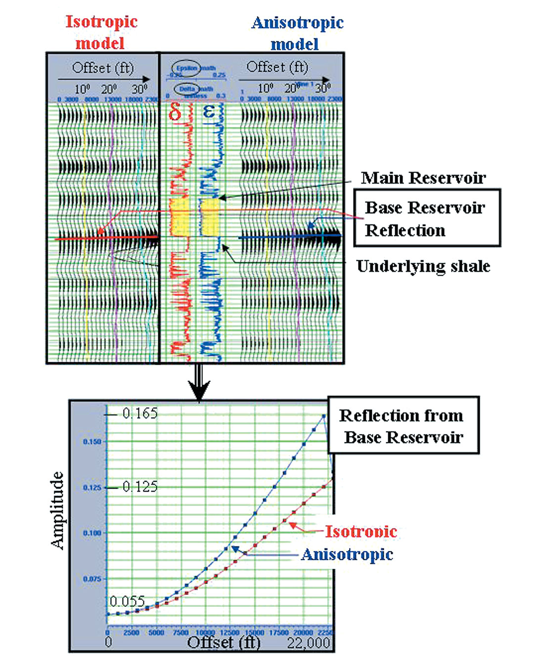
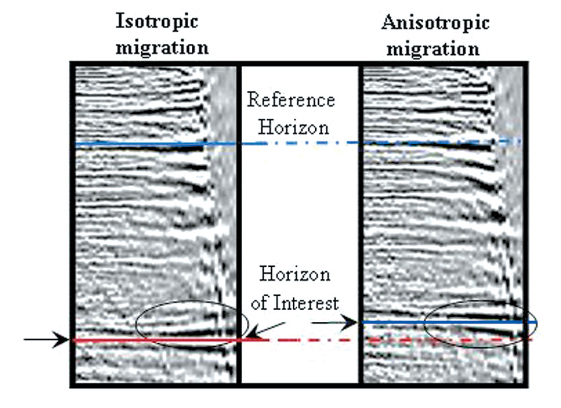
Figure 3 shows an example of a seismic gather from the same area as Figure 2, after PSDM using both an isotropic and a VTI algorithm. Naturally, with VTI-PSDM, the events are better positioned laterally. The VTI migrated gathers show events that are better flattened and where the energy is better focused. The final VTI migrated gathers exhibit a pull-up of approximately 1,000 feet (out of a total of approximately ~25,000 feet) from the isotropic migrated gathers. Furthermore, the increase in amplitude with offset at the base reservoir more closely matches that which was modeled with VTI-anisotropy in Figure 2. Seismic anisotropy, as characterized here, has a first order effect in the far offsets amplitudes at the base reservoir. It modifies very significantly the isotropic P-wave AVO of the zone of interest. It must be accounted for, if we hope to extract semi-quantitative properties of our reservoir from AVO information.

Conclusions: The quality of contemporary seismic data results from significant advances in acquisition and processing techniques, and has increased the demands on the seismic interpreter/analyst, who constantly tests the limits of existing technology in an attempt to decipher the message contained in every waveform.

The next level in Appraisal seismic analysis requires understanding quantitative changes in higher order wave propagation effects, such as anisotropy and attenuation in the context of bed tuning at seismic wavelengths. Such parameters were, until recently, impossible to recover, as their effects were buried within the ambient S/N of the data. Today, we can successfully identify the effects of transverse isotropy in a section, but we cannot quite yet quantify them in terms of changes in layer properties at the reservoir scale. Continued studies of converted waves, multi-azimuth seismology, and insights into the process of upscaling seismic rock properties, will lead to new breakthroughs in our quantitative understanding of seismically-derived Rock and Fluid properties at subsurface Conditions.

Jean-Pierre Blangy
BP, North America Exploration

Acknowledgements: I would like to thank BP management for permission to publish, BP’s seismic imaging group, and Leon Thomsen for kindly accepting to review the manuscript.

Question 3

Density Cube is supposed to help in avoiding low gas saturation pitfalls and find non-bright pays which may otherwise be difficult to find with conventional amplitude technology, and so significantly reducing risk in hydrocarbon exploration. Could you elaborate in detail how prospecting is done with the Density Cube, illustrating with examples how it qualifies the advantages mentioned above?

Answer

Density Cubes are seismic data volumes with values corresponding to subsurface density contrasts. Contrasts are the relative changes of a quantity, in this case density, across an interface such as the one formed between a reservoir and the cap rock which provides the seal. The observed strength or amplitude of seismic reflections are controlled by combinations of contrasts of the individual elastic parameters, Vp, Vs and density. Stacks of seismic data are dominantly governed by combinations of the contrast of P-wave velocity and density. Two-parameter AVO attributes are also controlled by combinations of two or more rock property contrasts. Using two-parameter AVO attributes and/or stack values, it is not possible to determine, without constraining assumptions, the contrasts of the three rock properties, Vp, Vs and density, individually.

Why is separating out the individual rock property contrasts, especially density, so important? As explorationists we are charged with relating the objective characteristics of seismic to subsurface properties such as lithology, reservoir properties and fluid type. Using amplitude and AVO attributes has provided some leverage but, as mentioned above, they are related to combinations of the individual rock properties. The traditional seismic parameters are oftentimes insensitive to changes in important parameters such as pay saturation and reservoir quality because of the their highly nonlinear dependence on those parameters. What can be done to provide an interpretation that is more sensitive to these important variables? The answer is simple. Fluid changes, and the most important lithology changes such as porosity and clay content variations, vary approximately linearly with density and density contrast. The same is certainly not true for their variation with Vp. The linear dependence of density, and hence density contrast, on pay saturation is well known compared with the highly non-linear relationship with Vp. The addition of small amounts of hydrocarbon can produce a large Vp contrast compared to the contrast from a fully saturated reservoir. This is not true for the density contrast. In many areas, particularly those where wet sands are similar in velocity to surrounding shales, the Vp contrast behaves non-linearly with respect to many of the lithology and fluid parameters we are most interested in. Density, on the other hand, almost always displays linear changes with the variations in subsurface lithology and fluid properties. Obviously if we could use a seismic volume whose amplitudes were a result of density variations only then our jobs as explorationists would be easier.

Density cubes provide a simple to use and efficient prospecting tool. They can be treated like any other seismic dataset. They can be interpreted easily and seamlessly within the 3D workstation project. All of the interpretation tools and data analysis tools found in the interpretation toolbox are applicable. Comparison with well data is substantially simplified compared with stack data and AVO attributes.

To demonstrate the advantages of using Density Cubes versus traditional volumes in the analysis of an area, three examples are provided to illustrate three categories of common exploration problems that show the advantages over traditional volumes.

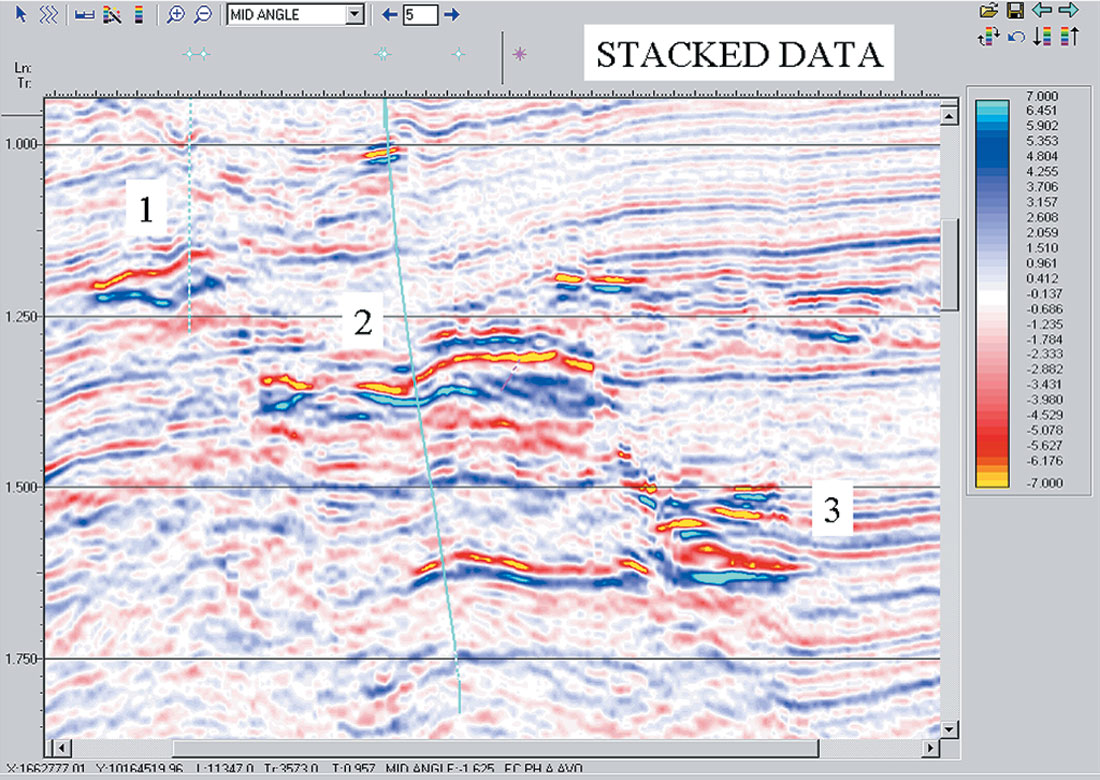
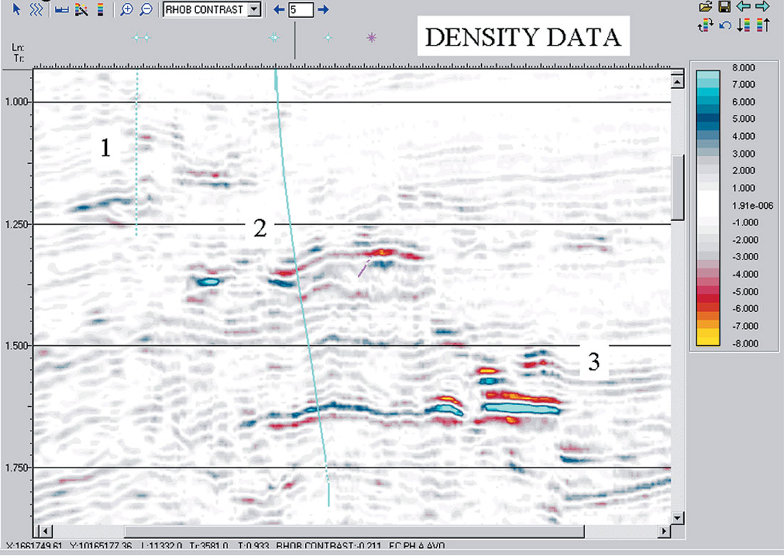
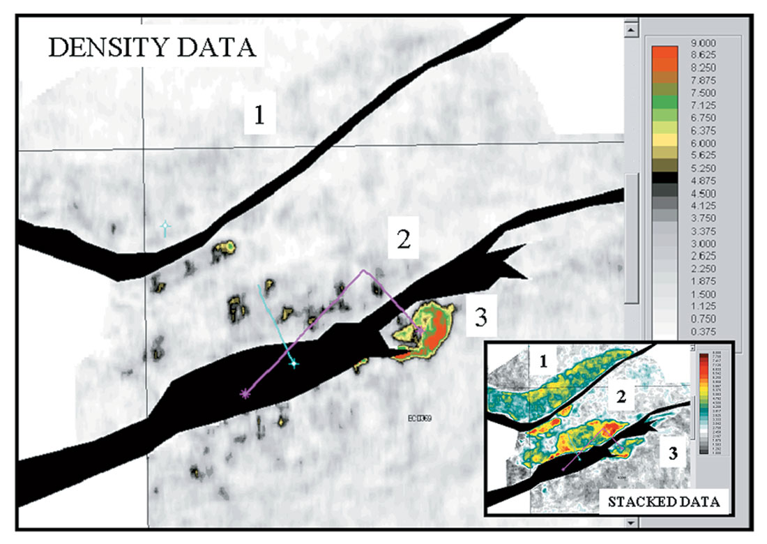
Example 1: Fluid Changes. Figure 1 is a stacked seismic section over three fault blocks. In this case, fault blocks 1 and 2 have already been drilled and found to contain excellent high porosity reservoir, but with uneconomic amounts of hydrocarbons. The amplitudes and anomalously slow velocity of the sands suggest water with low gas saturation as the fluid. The issue is whether or not to drill fault block 3. The stack amplitudes of Figure 1 shows little difference between fault block 2 and 3. Figure 2 is the same section extracted from the Density Cube. Although the color bars are different, the maxima and minima are close to the same. Notice how the density amplitudes associated with the two dry holes are very close to background in magnitude. The undrilled third fault block, however, has a very strong density contrast. Figure 3 is the horizon-based extraction from the Density Cube (the stacked amplitude extraction is in the inset for comparison). The magenta wells displayed on the map are two discovery wells that were subsequently drilled into fault block 3 and another density anomaly. Over 250’ of hydrocarbon- saturated reservoir were encountered in the first well that penetrated the mapped density anomaly.

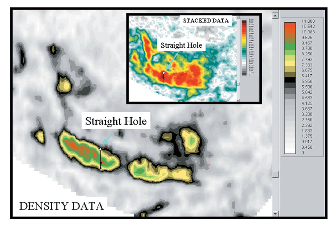
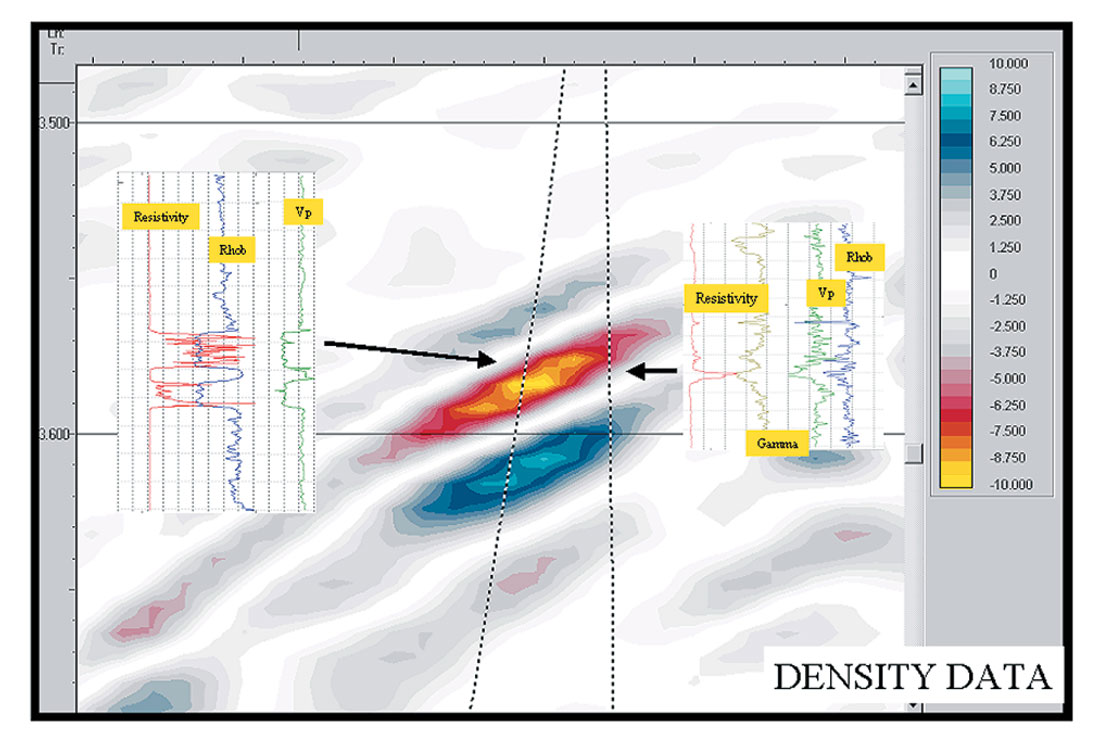
Example 2: Lithology Changes. Figure 4 shows an amplitude extraction from the Density Cube with the location of a straight hole plotted on it. The well placement was determined using the stacked amplitude dataset (see inset). Hydrocarbons were found in the first well, but the reservoir quality is not optimum even though the well was positioned to hit the stacked amplitude anomaly near a maxima. Examination of the extraction from the Density Cube shows that the well penetrated the reservoir on the edge of the density anomaly. A sidetrack was drilled using the density data and penetrated the heart of the density anomaly. Figure 5 exhibits an arbitrary line from the Density Cube that runs along the sidetrack. Logs from the two wells (displayed next to the wellbore) clearly show that thicker and cleaner reservoir was encountered in the sidetrack. The gradational reservoir found in the straight hole is probably associated with an overbank deposit, while the strongest part of the density anomaly pertains to the channel.

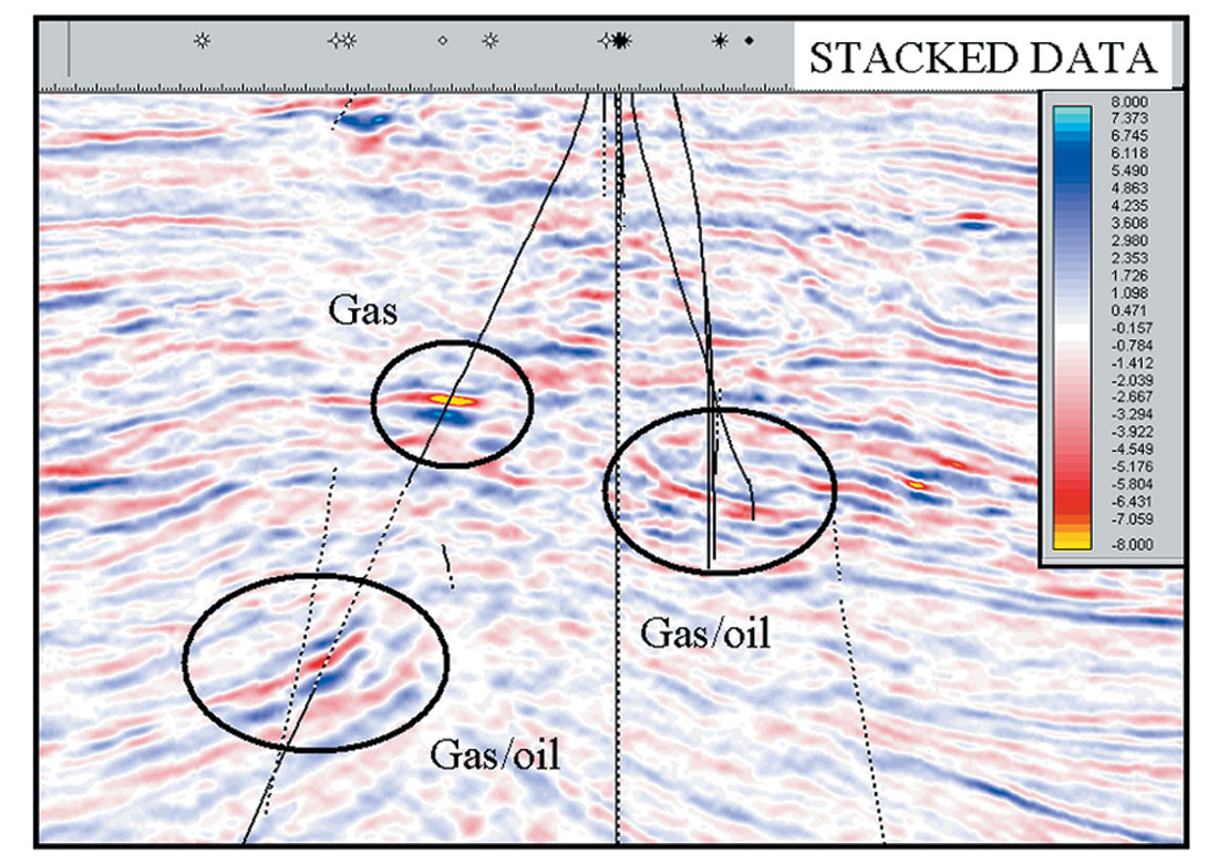
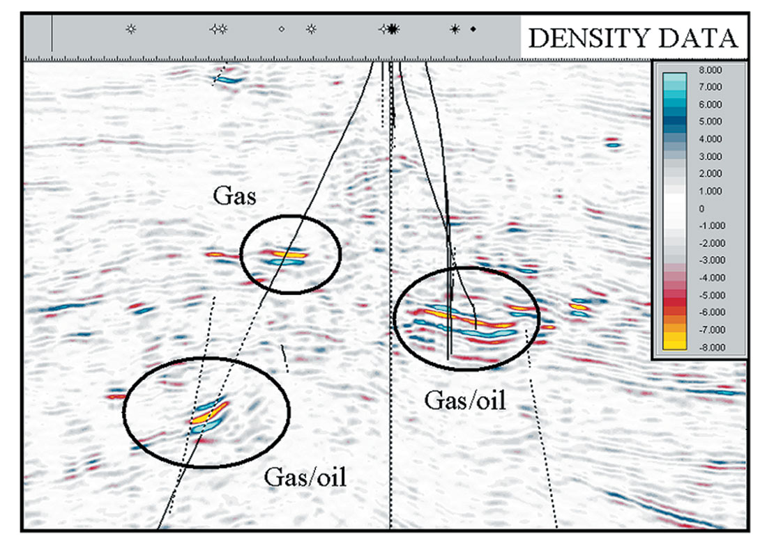
Example 3: Non-bright Pay. The term “non-bright” is at times a misnomer. There are many reasons why a hydrocarbon deposit may not result in strong seismic amplitudes. In this case we use non-bright to describe a reservoir that based on modeling should produce anomalous amplitude in the data, yet the stacked amplitude response is not very strong. Figure 6 shows a stacked amplitude section from a producing field. Only one of the three reservoirs circled exhibits anomalous amplitude. The reservoir sequence encountered is composed of stacked channels and overbanks with production coming from many levels. The shallowest of the reservoirs does produce amplitude and has hard shale as a top seal. The other two reservoirs have gradational interfaces and silty shales as the cap rock. Modeling suggests that the silty portions of the cap rock may contain some gas. In fact, there is a strong likelihood the entire section underneath the regional seal would be charged. The presence of the gas in the section will lower the velocity of all of the layers of various lithologies and remove much of the P-wave contrast between reservoir and cap rock. The stacked data, being dominantly driven by changes in P-wave contrast, will not be a good discriminator of high quality versus poor quality reservoirs. Figure 7 shows the same line extracted from the Density Cube. The three primary reservoirs now all show up as zones of anomalous density contrast (note the color scales are different, but the minima and maxima are the same). Similar to the previous example, the Density Cube is now highlighting the cleaner portions of the reservoir. The minor amounts of gas that percolate through the sequence are not enough to impact the density variations making the Density Cube a far better exploration tool in these circumstances.

These three examples were chosen to demonstrate the power and ease of working with density data. One must use caution, however, and realize that there are instances when density data alone will not tell the whole story. Both lithology variations and, at times, porosity variations can produce strong density contrasts. Using volumes driven by the contrast of the other elastic parameters, VP and Vs, or combinations thereof, can usually resolve these ambiguities. Density Cubes are still a form of seismic data. They have the same, and at times greater, sensitivity to noise and resolution issues as traditional seismic volumes such as stacks and 2-parameter AVO attributes, although patented methods are applied to reduce the instabilities. Prospecting using Density Cubes offers a lower risk, highly efficient tool for finding reservoirs, determining whether hydrocarbons are present and whether they are fully saturated.