The Duvernay Formation, located in central Alberta, Canada, is mainly an organic-rich shale that is a source rock for conventional oil and gas reservoirs, and more recently, also very attractive for exploitation as an unconventional shale play. The development of these types of plays requires the implementation of unconventional techniques, such as horizontal drilling and hydraulic fracturing, to increase the permeability of the reservoir. To assess the performance of a hydraulic fracturing stimulation, microseismic monitoring can be implemented to track fracture propagation and estimate the effective stimulated reservoir volume. The results of near-surface microseismic mapping, in a case study of a shale reservoir in the Kaybob-Duvernay formation, together with the available 3D seismic and well log data, are assessed to extract key characteristics of the reservoir and to forecast the hydrocarbon productivity after the hydraulic fracturing stimulation.
Introduction
Characterization of a typical oil or gas reservoir is comprised of integrating geological, geophysical and production data to determine its fundamental properties, such as porosity, permeability, fluid and organic content. These parameters can be estimated from conventional exploration methods including well logs and seismic reflection surveys. For unconventional reservoirs such as shale-gas or liquid-rich shale plays, where a hydraulic fracturing stimulation is required to enhance the reservoir productivity, additional techniques like microseismic monitoring are required to estimate the effectiveness of the stimulation. This paper outlines the implementation of a workflow to estimate the properties of a shale reservoir, and their implications for hydrocarbon productivity. The reservoir analyzed in this study is located in the Fox Creek region of Central Alberta, Canada (Figure 1). A well with four horizontal tracks was drilled through the Kaybob-Duvernay Formation in a north-south direction, and a multi-stage hydraulic fracturing stimulation was performed. The 3D seismic and the well logs from the vertical well shown in Figure 1 were also available for this case study to assist with interpreting the geological parameters of the reservoir.
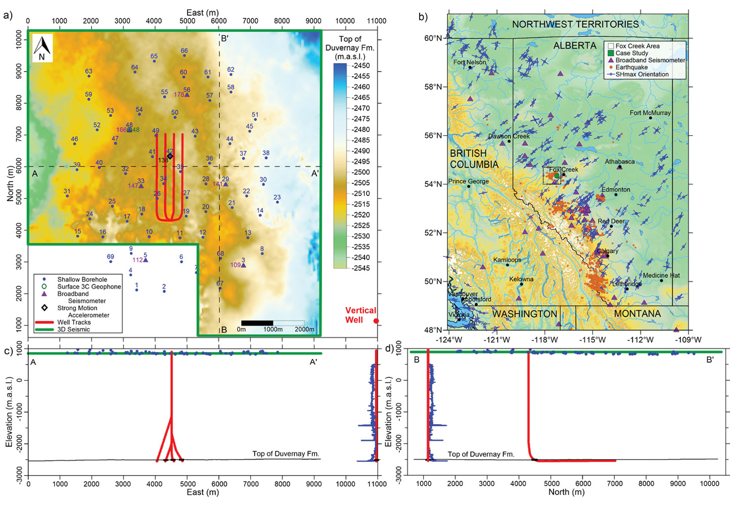
Due to the observed recurrence in recent years of anomalous seismicity associated with hydraulic fracturing operations in the Fox Creek region (Schultz et al., 2017), in the Kaybob-Duvernay zone it is mandatory to conduct seismic monitoring during any completion operations that include hydraulic fracturing (Alberta Energy Regulator, 2015). This stimulation was monitored using a shallow seismic array equipped with 69 conventional 3C short-period geophones, buried to a depth of 27 meters (see Figure 1a, c, and d). The recorded seismic data were processed to detect the microseismic events associated with the treatment. The results from the microseismic data, together with the available 3D seismic and well log data, were integrated to estimate the required parameters to forecast the production from the stimulated reservoir.
1. Well Log Data Analysis
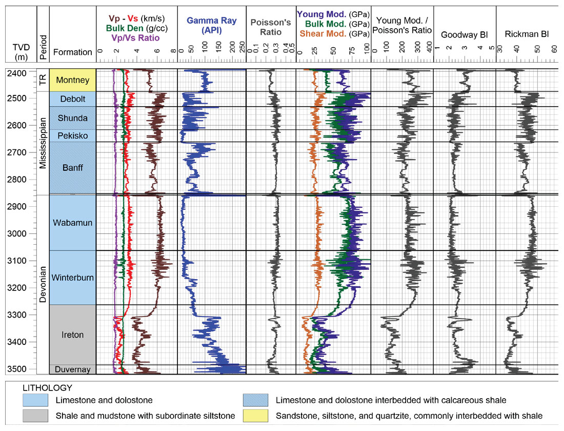
Figure 2 shows the dipole sonic, density, and gamma ray logs, together with the reported tops, from the vertical well shown in Figure 1a. The dipole sonic logs were used to produce a 1D laterally homogeneous velocity model to locate the epicenters of the detected microseismic events (discussed in Section 3), and the density log with the p- and s-wave velocities were used to calculate the dynamic elastic moduli logs following the seismic velocity equations for isotropic media (Mavko et al., 2009):
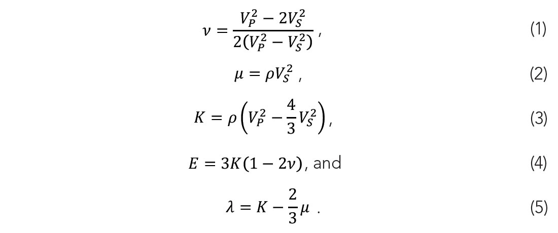
In these expressions, ν is the Poisson’s Ratio, μ is the Shear Modulus, K is the Bulk Modulus, E is the Young Modulus, and λ is one of Lamé’s elasticity constants. The brittleness logs shown in Figure 2 were calculated using three different equations based on the calculated dynamic elastic moduli. The first equation is the ratio between the Young’s Modulus and the Poisso's Ratio. The second equation is the Brittleness Index proposed by Goodway et al. (2010):

and the third equation is the Brittleness Index proposed by Rickman et al. (2008):

The gamma ray log starts to increase at 3305 meters depth due to the higher shale volume within the Ireton formation when compared with the upper calcareous units. At the Duvernay formation, reported at a depth of 3485 meters depth and 40 meters thick, the gamma ray log is even higher due to its higher total organic carbon (TOC) of 4.5% on average (Dunn, et al., 2012). The high gamma ray measurement – indicating high shale volume and TOC – and high Brittleness Index of the Duvernay Formation compared to the upper bounding formation, together with its potential to produce gas condensate due to its elevated pore pressure above the bubble point (Dunn, et al., 2012), make it a particularly attractive unconventional multiphase (gas condensate and natural gas) shale play for development (Alberta Energy Regulator, 2016).
2. 3D Seismic Interpretation
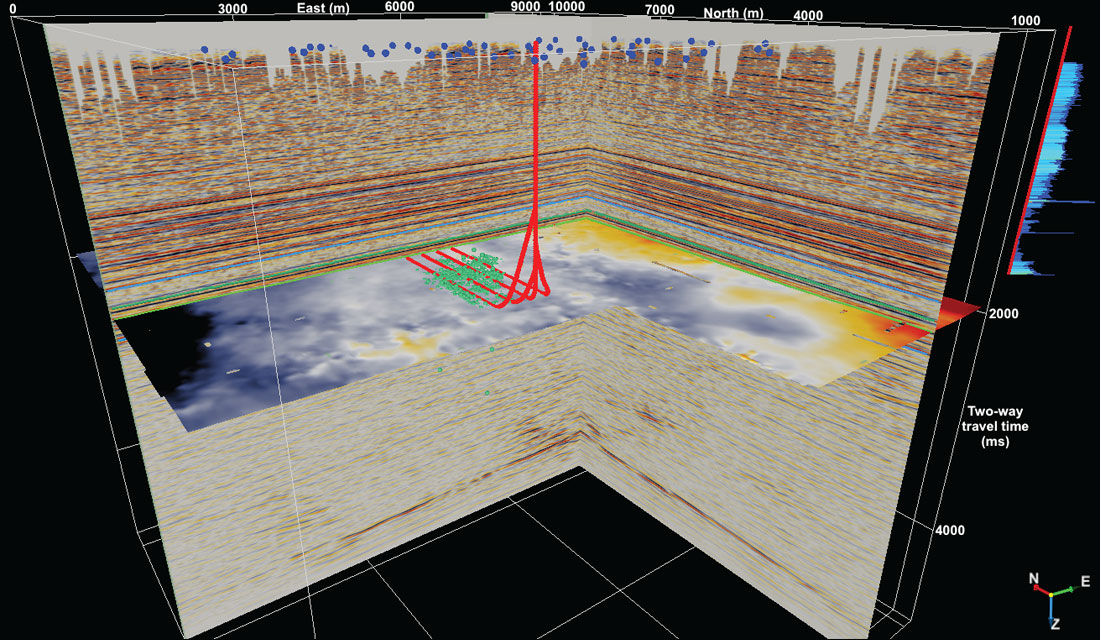
Figure 3 shows the pre-stack time migration (PSTM) for the 3D seismic survey shown in Figure 1a, with the horizontal treatment and vertical wells and the interpreted top of the Duvernay Formation. The shallow 3C seismic stations deployed for surface microseismic monitoring of the hydraulic-fracturing stimulation, and the microseismic events detected with this array (discussed in the following section) are also shown for reference. A velocity function was built for this two-way-traveltime horizon based on the depth of the top of the Duvernay Formation reported in the stimulated multi-horizontal well (tops shown in Figure 1c and d), and implemented for a time-to-depth conversion for the same horizon. This horizon, like all the upper horizons visible in the inline and crossline sections, is very flat and relatively homogeneous along the entire 3D seismic survey and does not suggest the presence of major faults in the reservoir. Only a slight increase of elevation is seen towards the northeast for the top of the Duvernay Formation.
3. Microseismic Data Processing and Interpretation
Some of the hydraulically fractured stages in the shale reservoir were monitored with the shallow 3C stations (shown as blue points in Figure 1a and in Figure 3). The processing of the recorded passive seismic data started with automatic detection of seismic events. It was based on a cross-correlation function that used a template event and extracted the P and S phase arrivals of the detected events. Around 4000 microseismic events were detected, using the implemented cross-correlation function, on the stages that were monitored. The dipole sonic log, from the vertical well next to the study area in Figure 2, was used as a velocity model to locate the epicenter of the detected events with P and S phase arrivals. The coda wave (or signal duration) and the radiated energy were also picked automatically for the same detected events. This information was used to estimate the (coda) magnitude and source radius of each event (Rodríguez-Pradilla & Eaton, 2018).
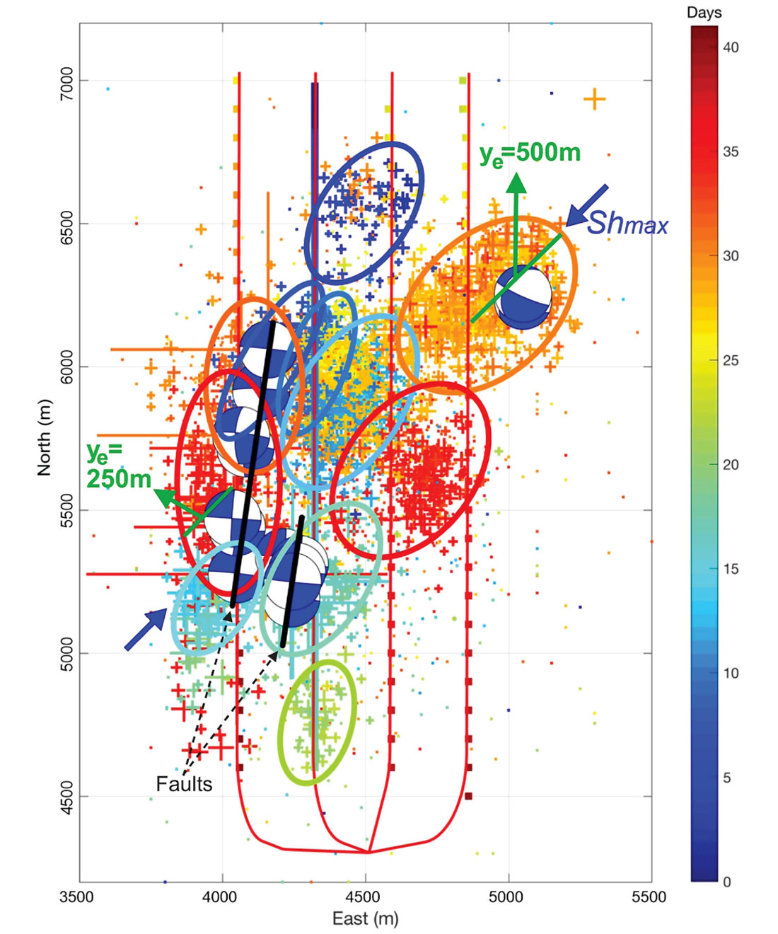
During the monitored stimulation, 17 seismic events with local magnitudes between 1.5 and 3.6 were also detected by the regional seismological network shown in Figure 1b, and reported in the Alberta Earthquake Catalogue (Stern, et al., 2018). According to the Alberta Energy Regulator’s Subsurface Order No. 2, any seismic event with local magnitude of 2.0 or higher within 5.0 kilometers of any stimulated well must be reported (Alberta Energy Regulator, 2015). Figure 4 shows the location and focal mechanism of these 17 events (reported by Zhang and Eaton, 2018), with the interpretation of two north-south faults that are inferred to be reactivated by the multi-stage stimulation. This faultreactivation process has been reported for similar hydraulic-fracturing stimulations in unconventional reservoirs in western Canada, and particularly for those located in the Fox Creek region (Bao & Eaton, 2016). The focal mechanisms of some of these events, together with the orientation of the maximum horizontal stress of the Fox Creek region (reported by Heidbach, et al. (2016) and shown in Figure 1b), indicates a strike-slip faulting mechanism for the induced events. This preference for strikeslip motions has also been reported for similar induced earthquakes in this region (Schultz, et al., 2017). The presence of these strike-slip faults, hardly visible in the 3D seismic survey due to their low vertical displacement (see Figure 5), determines the direction of fracture propagation in the shale reservoir during the stimulation.
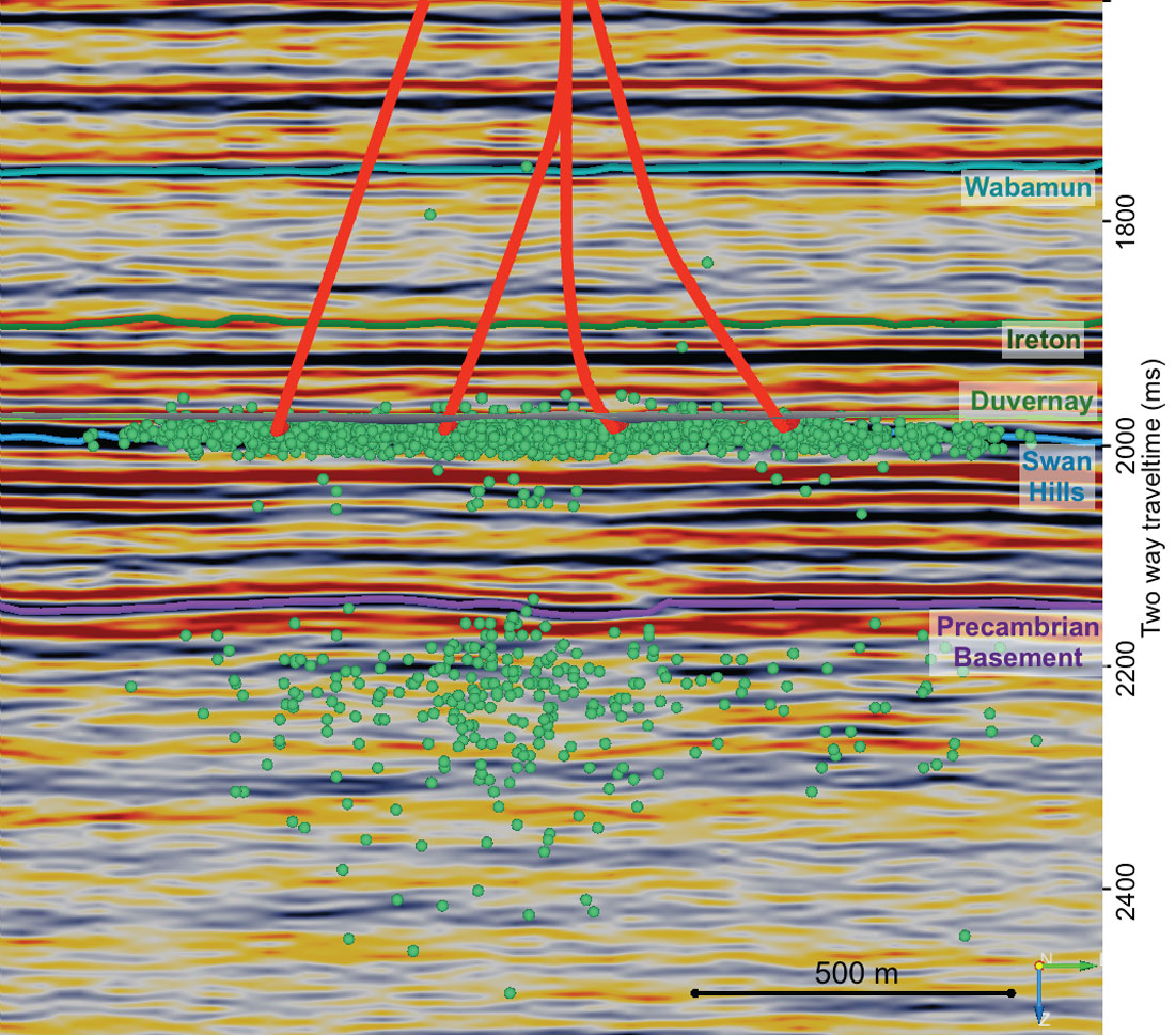
Figure 4 also shows the location and interpretation of the detected microseismic events (scaled by source radius) with the day of occurrence, where two different patterns are clearly visible. As expected, most of the hydraulically fractured stages show a fracture growth orientation that is aligned with the maximum horizontal stress, and the fracture half-distance (ye) for these stages can be easily measured based on the distribution of these events. However, the fracture growth of the stages nearby the interpreted north-south faults appear to be limited by them and follow a similar north-south orientation. Therefore, they have lower fracture half-distance compared with the stages farther from the fault. This difference in fracture half-distance caused by the fault reactivation has a major implication on the hydrocarbon production, as it defines the size of the stimulated reservoir volume on which the implemented production model (described in the following section) is based (Song and Ehlig-Economides 2011; Clarkson and Qanbari 2015).
4. Hydrocarbon Production Forecasting
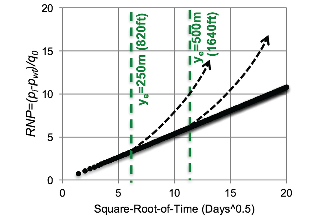
Several models can be implemented to forecast the hydrocarbon production of a reservoir, and several factors must be considered to determine the most appropriate method for each case. These factors include the type of reservoir (e.g. conventional oil/gas, tight oil/gas, fractured reservoirs), flow regimes (e.g. linear, elliptical, boundarydominated), the type of the simulation (i.e. analytical, semi-analytical, or numerical), and the available data from the reservoir. For this case study, the linear-to-boundary flow model (LTB) proposed by Wattenbarger et al. (1998) for tight-gas reservoirs, and modified by Clarkson and Qanbari (2015) for multifractured tight light-oil reservoirs with multiphase flow (as the expected condensate/gas flow from the Kaybob-Duvernay Formation), was implemented. This LTB model defines the Rate-Normalizing-Pressure (RNP) as a stabilizing function to linearize the declining curves of the reservoir pressure and flow rate against the square root of time (from Song and Ehlig-Economides, 2011):

where pi is the initial reservoir pressure in psi, pwf, is the well flowing pressure in psi, and q0 is the oil-phase flow rate in Stock Tank Barrel per Day (STB/D). The initial stabilized production of a hydraulicfractured reservoir, as tight-oil or tight-gas reservoir, will remain linear until the reservoir pressure reduction reaches the boundary of the fractured reservoir. The time when the end of the linear flow (telf) occurs on the oil phase can be calculated with the following expression (from Clarkson and Qanbari, 2015):

where ϕ is the reservoir porosity, μoi is the oil viscosity in centipoise (cp), koi is the permeability of the stimulated reservoir in millidarcies, cti is the rock compressibility in 1/psi, and ye is the fracture half-distance in feet. After telf, the stabilized production function increases exponentially. The following expressions (from Clarkson and Qanbari, 2015) can be implemented to calculate the oil-phase flow rate (q0) before and after telf :
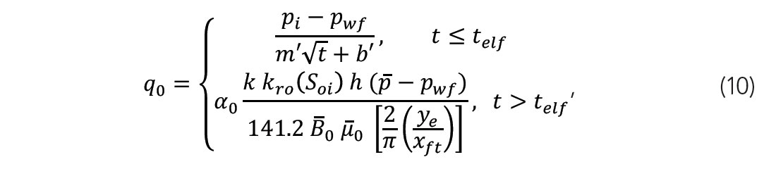
where m’ is the slope of square root of time plot in psi/STB/√day, and b’ is the intercept of square root of time plot in psi/STB. This LTB model can be adapted to multiphase condensate/gas reservoirs by employing a low viscosity for the oil phase (μoi) to simulate the gas condensate flow (e.g. 1 centipoise), and a constant condensate-gas ratio (CGR) to obtain the gas-phase flow (qg) from the calculated oil-phase flow before telf (Clarkson, et al., 2014). For the Kaybob-Duvernay Formation, the reported final CGR range between 0 and 400 barrels of condensate per million standard cubic feet of natural gas (STB/MMcf), and wells with a CGR below 50 STB/MMcf are assumed to be primarily natural gas wells (Alberta Energy Regulator, 2016).
| NOMENCLATURE | PARAMETER | VALUE | SOURCE |
|---|---|---|---|
| Table 1. Input data for the simulated linear flow. | |||
| z | Reservoir depth (m) | 3485.0 | From well log data, Figure 2 |
| pi | Initial reservoir pressure (psia) | 5030.8 | Assumed Hydrostatic Pressure, 0.44 psi/ft |
| T | Reservoir temperature (ºF) | 220.2 | Geothermal gradient: 30 °C/km. Source: Bachu, S., 1994 |
| pwf | Well flowing pressure (psia) | 1000.0 | Source: Clarkson & Qanbari, 2015 |
| k | Permeability (millidarcy | 1.0 | Assumed value for the fractured region of the reservoir |
| φ | Porosity (fraction) | 0.1 | Source: Dunn et al., 2012. |
| cti | Rock compressibility (1/psi) | 0.00002 | Source: Clarkson & Qanbari, 2015 |
| h | Formation thickness (ft) | 131.2 | From well log data, Figure 2 |
| ye | Total fracture half-distance (ft) | 820 / 1640 | From microseismic data, Figure 4 |
| m' | Slope of square root of time plot (psi/STB/√day) | 0.6 | Source: Clarkson & Qanbari, 2015 |
| b' | Intercept of square root of time plot (psi/STB) | 0.0 | Source: Clarkson & Qanbari, 2015 |
Conclusions
The Duvernay Formation is an organic-rich formation highly attractive for unconventional shale development, especially in the Kaybob area where this case study is located due to its potential to produce both gas condensate and natural gas. The implemented linear model for the expected multiphase flow (liquid and gas) is based on the reservoir properties obtained from seismic, microseismic, and well log data. Several reservoir characteristics required as input parameters for the production forecasting had to be assumed. They were taken from similar shale reservoirs with reported data due to the current lack of data from the reservoir in this study. These values were used as the initial reservoir pressure or taken from laboratory measurements done on core samples. The end of the linear flow regime ( telf ) was calculated for two fracture half-distances obtained from the microseismic data by assuming a permeability for the stimulated reservoir, and a low oil viscosity for the estimated reservoir temperature to simulate the condensate flow. The measurement of telf from real production data can be implemented to estimate more accurately the permeability of the stimulated reservoir, and to forecast the non-linear hydrocarbon production of the reservoir after telf .

Acknowledgements
The author wishes to express his thanks to the Natural Science and Engineering Research Council of Canada (NSERC) who provided financial support (grant IRCPJ/485692-2014), as well as to all the sponsors of the Microseismic Industry Consortium for their ongoing support. TransAlta Corp. and Nanometrics Inc. are also thanked for providing the reported seismicity detected with the regional seismological network installed in Alberta and the surrounding areas, and the operating companies of the studied shale play for providing the well logs and for supporting the near-surface monitoring program acquired under license using MicroSeismic Inc.’s BuriedArray® design. Finally, we thank Ron Weir from the University of Calgary for providing the interpretation of the top of the Duvernay Formation from the 3D seismic dataset.


Join the Conversation
Interested in starting, or contributing to a conversation about an article or issue of the RECORDER? Join our CSEG LinkedIn Group.
Share This Article