Recently two papers were published in the RECORDER that dealt with a comparison of Megabin geometry with orthogonal geometry in the context of 5D interpolation (Duncan et al., 2014; Harger and Schweigert, 2014). What struck me is the use of coincident shots and receivers in the Megabin geometries and also in the orthogonal geometry discussed in Duncan et al. Perhaps not so surprising for the Megabin geometry as it is according to the original recipe given in Goodway and Ragan (1998). Cooper and Egden (1999) describe another comparison between Megabin and orthogonal geometry. In their paper shots and receivers of the Megabin geometry do not coincide.
The use of coincident shots and receivers surprises me because of the emphasis by many survey designers (as in Cooper and Egden, 1999) on unique fold: traces with absolute offsets differing less than a small amount are considered to be redundant. When coincident shots and receivers occur in a geometry, there are invariably traces (reciprocal traces) with exactly the same absolute offset and with opposite azimuth, which is the ultimate redundancy.
In an earlier note (Vermeer, 2013) I denounced the use of unique fold as a quality measure of an acquisition geometry, because traces with nearly the same absolute offset but with different azimuth tend to have their own requisite role and are valuable members of the total geometry. However, reciprocal traces are not valuable in general.
In this paper I focus on the effect of coincident shots and receivers on effective fold and on data quality. I do this in the context of what constitutes a good acquisition geometry; therefore I start with a brief description of such a geometry (much more detailed descriptions can be found in Vermeer, 2010 and 2012) followed by a brief discussion of the Megabin geometry. The second part of this paper then looks at the effect of coincident shots and receivers and looks as well at alternatives, both for Megabin geometry and orthogonal geometry.
Characteristics of a good acquisition geometry – 3D symmetric sampling
3D symmetric sampling is based on the reciprocity theorem, which leads directly to the consequence that shot and receiver sampling should be the same. Ideally, the same sampling interval should be used for all four horizontal shot (subscript s) and receiver (subscript r) coordinates, or Δxs = Δxr = Δys = Δyr. If applied, the resulting geometry may be called full 3D. Another requirement is that sampling intervals should be small enough for alias-free sampling. We may aim for alias-free sampling of the whole wavefield, or for alias-free sampling of only the desired wavefield.
Normally, alias-free sampling of the desired wavefield, let alone the whole wavefield, is way too expensive. As a compromise two of the four spatial coordinates may be sampled alias-free leading to properly sampled 3D subsets of the 5D wavefield. In orthogonal geometry, the other two spatial coordinates are the line intervals of that geometry. The line intervals determine the sparsity of the geometry (Vermeer, 2010). Less sparsity, i.e., smaller line intervals, leads normally to better final data quality.
Apart from the four spatial coordinates, the designer has to select the maximum shot-receiver offset in x and in y, or the maximum inline and crossline offsets. These maximum offsets depend on maximum depth of interest and on processing requirements, such as AVO, azimuthal analysis, and full-waveform inversion. A completely symmetric geometry with equal maximum inline and crossline offsets and equal shot- and receiver-line intervals is ideal, but there may be practical and/or budgetary reasons to deviate from the ideal.
| Parameter | Symbol | Regularity requirement |
|---|---|---|
| Table 1. Regular orthogonal geometry fully described by six parameters (adapted from Vermeer, 2012, Table 4.1) | ||
| Receiver-station interval | Δr | |
| Shot-station interval | Δs | |
| Receiver-line interval | RLI | = nS × Δs |
| Shot-line interval | SLI | = nR × Δr |
| Receiver-spread length | LR | = 2 Xmax,i = 2 Mi × SLI |
| LS | = 2 Xmax,c = 2 Mc × RLI | |
The above requirements are not sufficient yet for a good acquisition geometry. Table 1 describes additional requirements, where nS is number of shot locations between each consecutive pair of receiver lines, nR is number of receiver locations between each consecutive pair of shot lines, Mi is inline fold, Mc is crossline fold, Xmax,i is maximum inline offset, and Xmax,c is maximum crossline offset. These requirements lead to a regular geometry in which total fold M is constant in the fullfold area of the geometry. Note that regular geometry requires centre-spread acquisition with an even number of active receivers in the receiver spread and those receivers must be listening to an even number of shots in the shot spread. Note also that spread length is defined as number of receivers times station interval (Vermeer, 2012, Appendix B).
The prescription of regularity means that 1) each cross-spread can be split into exactly M unit-cell sized tiles called offset-vector tiles (OVT) and 2) the M-fold geometry can be split into M different singlefold OVT gathers (also known as COV gathers, Cary, 1999). Each one of those gathers should be able to produce a prestack migrated image of the subsurface in the fullfold area of the geometry. The quality of the images depends on the station intervals and also on the line intervals. The symmetry of the cross-spread ensures that pairs of OVT gathers called reciprocal OVT gathers help to mitigate the sparsity of the geometry and to reduce acquisition footprint (Vermeer, 2007). Reciprocal OVTs do not have reciprocal traces but consist of traces in opposite quadrants of the cross-spread with the same range of absolute inline and absolute crossline offsets. OVT gathers are also useful for velocity analysis (Guillaume et al., 2010), for analysis of azimuthal anisotropy, and for other applications (Vermeer, 2012).
In practice, completely regular geometries are never acquired because there are always obstructions that force shot and receiver locations to deviate from the nominal positions. Yet, it is important to know what is the ideal acquisition geometry, to strive for it in the field and then use various processing techniques to correct for the deviations as much as possible.
Megabin geometry
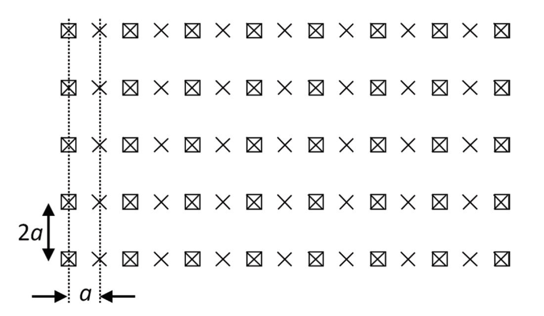
Megabin geometry, as patented by Goodway and Ragan (1998), also recognizes that alias-free sampling of all four spatial coordinates is too expensive. The compromise in Megabin geometry is to sample coarser in the crossline direction than in the inline direction. For inline receiver station interval a, the crossline station interval (or receiver line interval) equals 2a, whereas the shot station intervals are equal to 2a in inline as well as in crossline direction (Figure 1). Shot and receiver stations are arranged along the same lines, whereas all shots coincide with as many receivers. Essentially, this is an implementation of parallel geometry with crossline binsize being twice as large as inline binsize and necessitating interpolation in the crossline direction to arrive at square bins.
The coarse crossline binsize is the weak point of the Megabin design, as also agreed by the inventor (Goodway, 2013). Often the crossline binsize is the weak point in parallel geometry, because this binsize depends on line interval: line intervals have to be small for a proper crossline binsize needing almost unlimited access. Yet, Megabin geometry has also some advantages; in agricultural areas it may be much easier to lay out only parallel lines rather than also orthogonal lines (Norm Cooper, 2014, personal communication). Another advantage is the small size of the OVTs of this geometry which is equal to the grid size of the shots (2a x 2a). Schmidt et al. (2009) applied OVT processing to a Megabin survey. In orthogonal geometry the size of the OVTs is determined by the line intervals, which are usually much larger than twice the station intervals. Only for shallow targets, complex geology, or complex near surface may it be necessary to use very small line intervals in orthogonal geometry with similar values as in Megabin. Seeni et al. (2010) describe the acquisition of an orthogonal geometry in Qatar with 120 m receiver-line intervals, 90 m shot-line intervals, and 7.5-m station intervals for both shots and receivers.
Perhaps the main reason that Megabin has been successful in the Western Canadian Sedimentary Basin is the very benign geology (Schmidt et al., 2009). Aliasing of the data only occurs for noise (that is often not all that serious) and in the desired wavefield only prior to the NMO correction. After NMO correction only diffractions may be aliased with coarse sampling. Application of the Megabin geometry in other areas with more geologic and near-surface variation (such as Foothills) would be more problematic.
Fold variations and reciprocal traces – Megabin
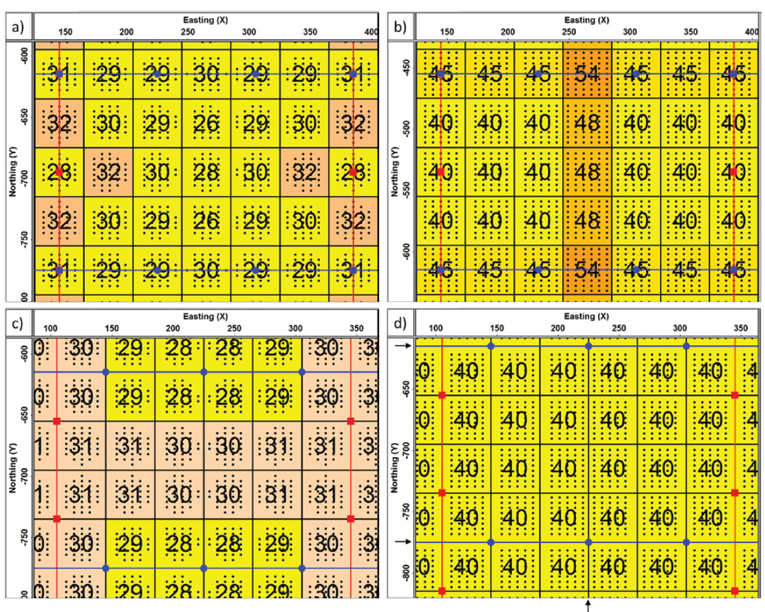
For the analysis of the Megabin geometry, I select for the receivers an inline interval of 60 m and a crossline interval of 120 m. The shots are located in a square grid of 120 x 120 m, initially along the receiver lines and even coinciding with receivers, but I look as well at other shot-receiver arrangements. The binsize of all arrangements is 30 m inline and 60 m crossline. Some of the geometries discussed in the referenced papers on Megabin have been acquired with all receivers live, followed by selecting all traces with a radius around each shot equal to the maximum offset for the level of interest. Here, the aim is to get regular geometry with regular fold in the fullfold area of that geometry; this requires the use of a rectangular template. The template is rolled with each shot.
In my example of Megabin geometry the template consists of 17 receiver lines listening to each shot (including the line on which the shot is located) with 33 receivers in each line (including one at the shot location). This means that the maximum inline (and crossline) shot-receiver offset is exactly 960 m.
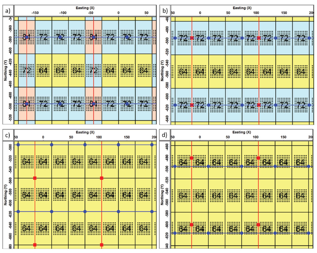
Figure 2a shows some bins of the first arrangement, together with the fold in each bin and an array of black circles representing the offset-vector distribution. The shot lines are drawn vertically as red lines and the horizontal blue lines are the receiver lines (and are considered as shot lines as well in actual practice). The unit cell of this geometry consists of 8 bins. The bin at the intersection of a shot line and a receiver line has 9 x 9 = 81 fold; the other bins along the shot and receiver lines have 8 x 9 or 9 x 8 = 72 fold. The yellow bins have 8 x 8 = 64 fold. Clearly the total fold of this geometry is not constant in the fullfold area, so it cannot be called regular geometry.
Perhaps more disturbing is the occurrence of reciprocal traces caused by coincident shots and receivers. Every pair of coincident shots and receivers produces two traces for which shot and receiver location are interchanged. Knapp (1985) already argued that shots should not be located at group centres, but midway between consecutive group centres. His main argument was that ground roll of such pairs of traces tends to be the same and will not be suppressed in stacking. Another argument might have been that the (P-wave) raypaths of interchanged shot and receiver pairs are identical providing the same information about the subsurface. Acquisition money can be spent better. Knapp’s discussion was about the acquisition of 2D data. In 3D there is another negative effect, which is that the number of unique traces varies drastically from bin to bin.
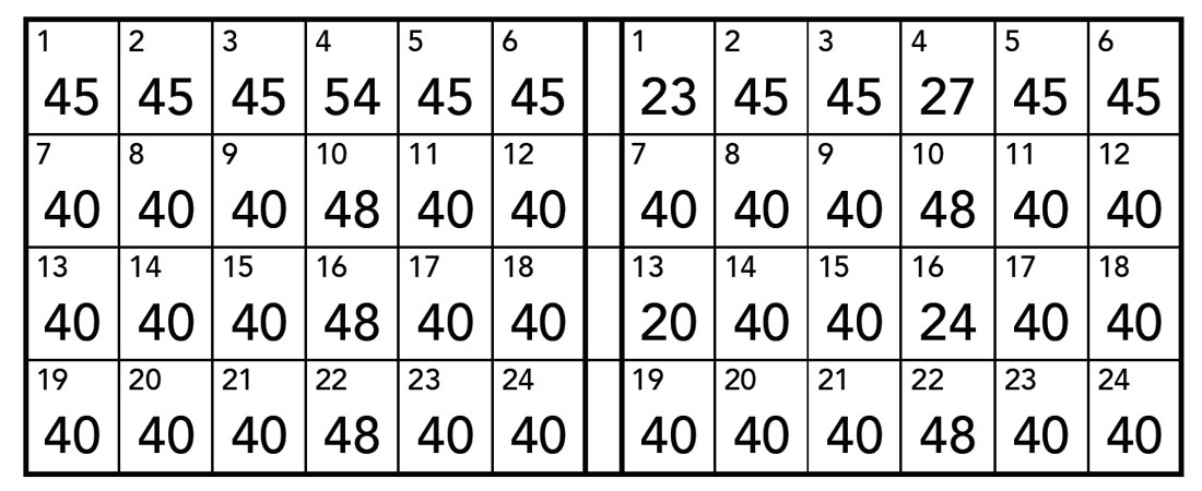
Table 2 compares the fold of the 8 (numbered) bins of the unit cell before and after discarding the redundant traces. About half the traces in four of the eight bins are redundant. Bin 1 is right at the intersection of a receiver line with the shot line. Eighty traces in this bin are reciprocal to another trace, only the zero-offset trace is not reciprocal to another trace; therefore, there are 41 unique traces and 40 traces that may be discarded because they do not provide new information, i.e., they are redundant. In bins 3, 5, and 7 all traces occur in pairs, whereas in the other bins no reciprocal traces occur. The number of reciprocal traces corresponds with what can be predicted a priori: one half of all receivers listening to a shot are also shot locations; therefore 50% of all traces is reciprocal and 25% is redundant.
There is no need to reject Megabin because of all reciprocal traces: Shifting the shot locations to positions halfway pairs of receivers eliminates the occurrence of redundant traces. Cooper and Egden (1999) use this kind of Megabin implementation. Figure 2b shows that shifting the shot location in this way does not yet lead to regular fold. The template of this Megabin implementation is similar as for Figure 2a with 9 receiver lines listening to each shot; only the number of receivers in each line is now equal to 32. This produces a constant inline fold of 8 (8 black circles in the inline direction in each array of circles), but the crossline fold varies between 8 and 9. To create regular fold it is best to locate all shots halfway the receiver lines with 16 receiver lines listening to each shot (Figure 2c). Unfortunately, this eliminates one of the advantages of Megabin geometry: needing access only along rather widely spaced parallel lines. Figure 2d illustrates an implementation with the shots closer to the receiver lines, thus reducing access requirements, but this leads to some extra asymmetry of the 3D shot gathers in the crossline direction (there is already the asymmetry of the receiver crossline sampling interval being twice the inline sampling interval). This asymmetry produces OVTs that are not exactly reciprocal in opposite quadrants.
Fold variations and reciprocal traces – orthogonal geometry
Duncan et al. (2014) compare Megabin with orthogonal geometry data. All data are extracted from a much denser survey. In the original survey coincident shots and receivers were used and these are also present in the Megabin and orthogonal geometry being compared. In their orthogonal geometry shot and receiver station intervals are 80 m with nR = 3 and nS = 2. For the sake of checking the regularity of this geometry I selected a template with 31 receivers per receiver line, with 17 active receiver lines for the shots coincident with a receiver, and with 16 active receiver lines for the shots halfway the receiver lines. Figure 3a,b show analyses focusing on the 24 bins of one unit cell of this geometry. Figure 3a represents all traces with offsets smaller than 1200 m, whereas Figure 3b shows all traces of the described templates.
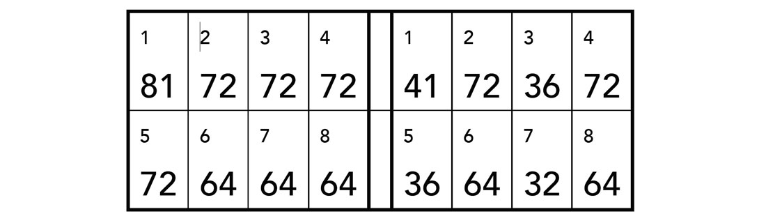
Also in this orthogonal geometry reciprocal traces occur. One out of two shots coincides with a receiver and one out of three receivers coincides with a shot, or one sixth of all traces is reciprocal. Table 3 illustrates how reciprocal traces are distributed across the 24 bins of the unit cell: Bins 1, 4, 13 and 16 consist mostly of reciprocal traces whereas the other 20 bins have none. About 8% of all traces are redundant. Of course, the redundancy also occurs in the corresponding bins of Figure 3a.
Figure 3c and 3d illustrate the offset distributions for the equivalent geometry without any redundant traces. Now fold is constant at 40, whereas the offset-limited folds in Figure 3c vary less than in Figure 3a.
Discussion
For P-waves reciprocal traces give information about the subsurface that is identical. Of course, for converted waves with P-wave down and S-wave up, the raypaths are not the same and any recorded C-wave energy would not be the same between reciprocal traces. Yet, even if the aim of the acquisition is to acquire C-waves, then P-waves are normally of interest as well, and more information about the subsurface will be gathered by never using coincident shots and receivers.
It may also be argued that interchanging shot and receiver locations when using buried dynamite would not strictly produce reciprocal traces: one would need a surface source (impossible with dynamite) and a buried receiver for reciprocity. Yet, the far fields of the shot-receiver pairs would still be very similar. [It would be very instructive if the reciprocal traces used in Duncan et al. (2014) were analyzed for their similarity, especially outside the ground-roll cone.]
I cannot see any good reason to use coincident shot and receiver locations. Granted, the acquisition of zero-offset traces with coincident shots and receivers looks attractive; however, when the acquisition lines intersect halfway station centres, each zero-offset trace is replaced by four near zero-offset traces, which may be considered ample compensation (compare Figure 3a with Figure 3c). Coincident shots and receivers also lead to pairs of reciprocal traces that may record similar noise and give rise to extra acquisition footprint, whereas seismic amplitudes to be measured for AVO are not sampled at as many offsets as in an equivalent geometry without any coincident shots and receivers.
Goodway (2013) states there is “extremely erratic offset and azimuth sampling” in routine 3D acquisition. This may be true for absolute offset, but Figure 2 and Figure 3 show that inside bins the offset-vector distribution is always extremely regular for inline and crossline distributions. On the other hand, there is no doubt that bin-to-bin variations in offset distribution tend to be stronger the larger the number of bins in a unit cell. It is of interest to look a bit closer at those bin-to-bin variations in the offset distribution.
Orthogonal geometry can be considered a collection of overlapping midpoint areas of cross-spreads. Inside each cross-spread bin-to-bin variations are minimal, because neighbouring bins in the inline direction all share the same shot and have been recorded by neighbouring receivers and neighbouring bins in the crossline direction share the same receiver that has listened to neighbouring shots. The real problem is the cross-spread edges. Figure 3d may be used to illustrate this problem. The arrows indicate where the bin-to-bin variation is significant. Across the indicated vertical line, the array of offset vectors jumps most in the inline direction. Across the receiver lines, the array of offset vectors jumps most in the crossline direction. Everywhere else the bin-to-bin variation is minimal. The location of the discontinuities depends on inline fold (odd in this case) or on crossline fold (even in this case). The inline discontinuities occur where one shot line with its cross-spreads stops contributing and another shot line starts contributing to the bins. In other words: the discontinuities correspond to the cross-spread edges.
There are two main strategies to counter this effect. First, reduce the line intervals in orthogonal geometry, thus reducing the size of the unit cell, and second, a regular geometry should be designed with reciprocal OVTs that mitigate the effect of the sparsity of the geometry (Vermeer, 2007, 2010, 2012). Figure 2c and Figure 3d illustrate that regular geometry is only obtained if shot and receiver lines intersect each other halfway between shot and receiver stations.
It may be argued that regular geometry is fine for deep targets where all offsets may contribute to the final image, but not for shallower objectives where offset limitation has to be applied. However, it is still advantageous to migrate all OVT gathers separately and to determine afterwards from what time onwards a gather with large average offset may contribute to the final product. This approach ensures that final amplitudes of the stacked migrations are not dependent on fold variations.
Another advantage of focusing on proper sampling of two spatial coordinates only rather than on trying to sample all four coordinates equally well as in Megabin geometry is that fine sampling of the cross-spreads allows better prestack processing results, in particular prestack noise removal. The use of smaller bins is often the first step towards better processing, imaging and interpretation results.
Conclusions
3D seismic survey design of orthogonal geometry should aim for regular geometry with symmetric cross-spreads. The geometry can be split into as many offset-vector tile gathers as the total fold of the geometry allowing optimal velocity analysis and imaging. Reciprocal traces should never be acquired as they provide redundant information, whereas reciprocal offset-vector tiles mitigate each other’s acquisition footprints. The footprints are reduced further by choosing smaller line intervals.
Megabin if used should have shots located between receivers, thus avoiding acquisition of reciprocal traces. Even then, the bins are necessarily too large (mega) for optimal results as the aim of choosing this geometry is not to discriminate between the four spatial coordinates. Dense sampling of only two coordinates as in orthogonal geometry allows coverage of the whole survey area in an affordable way with densely sampled midpoints for optimal imaging results.

Acknowledgements
Thank you to Jeff Deere for his review of this paper. The analyses presented in Figures 2 and 3 were made with Omni 3D survey design.


Join the Conversation
Interested in starting, or contributing to a conversation about an article or issue of the RECORDER? Join our CSEG LinkedIn Group.
Share This Article