The Peace region of NE British Columbia is an important agricultural area. It also contains significant gas reserves in the Montney natural gas play area. Agriculture and gas production require considerable volumes of water. There are also communities and First Nations within the region that require potable water for domestic use. A large component of the Peace region’s water comes from groundwater. Specific groundwater investigations have been undertaken in the region; for example the integration of ground EM, seismic and borehole logging (Hickin and Best, 2013 and Hickin et al., 2016). These are site specific and do not provide the regional overview that is needed to assess the availability of water in the region.
The Peace project is a collaborative project involving Geoscience BC, the BC Ministry of Forests, Lands and Natural Resource Operations, the BC Ministry of Environment, the BC Oil and Gas Commission, the BC Ministry of Natural Gas Development, Progress Energy Canada Ltd., and Conoco Phillips Canada, with additional support from the Peace River Regional District and the Canadian Association of Petroleum Producers. The objectives of the project are to provide knowledge on water availability (volume and location), water quality, and recharge. One of the objectives is to provide a regional overview of Quaternary and shallow bedrock aquifers within the Peace region. This paper presents the results of a regional study integrating more than 1200 gamma logs with an airborne electromagnetic (AEM) survey that partly addresses this objective.
Location of project area within the Peace region
Figure 1(a) is a map showing the project area (outlined as a black rectangle) with several areas outlined in green that were added after consultation with First Nations and local municipalities. The underlying map shows the main roads, rivers, and drainage systems. The area covers a large portion of the Peace region from just north of Fort Saint John to slightly north of Pink Mountain.
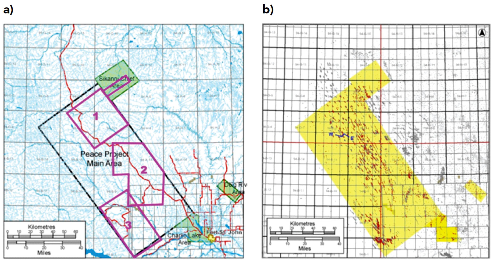
Gamma log data
Petrel Robertson applied a statistical method (Quatero et al., 2014) to correct for casing and cement attenuation in the near-surface section of gamma logs for approximately 1200 petroleum wells (Petrel Robertson, 2015). The gamma logs, along with usable water well logs, were interpreted by Quaternary Geosciences Inc. to provide depth to bedrock and potential sand/ gravel aquifers within the Quaternary section of the project area (Hayes et al., 2016). Figure 1(b) is a plot showing the location of petroleum wells within the Peace region. The red coloured wells were those used in this study. Figure 2 is a cross section from the corrected gamma logs (shown in Figure 1(b) as W – E in the northwest quadrant). The red curves are the corrected gamma logs and the black curves are the gamma logs before corrections were applied. After correction, the change in magnitude observed at the bottom of the casing on the uncorrected gamma logs vanishes. The wavy line is the interpreted top of bedrock. Datum was set at the top of the Sikanni Formation.
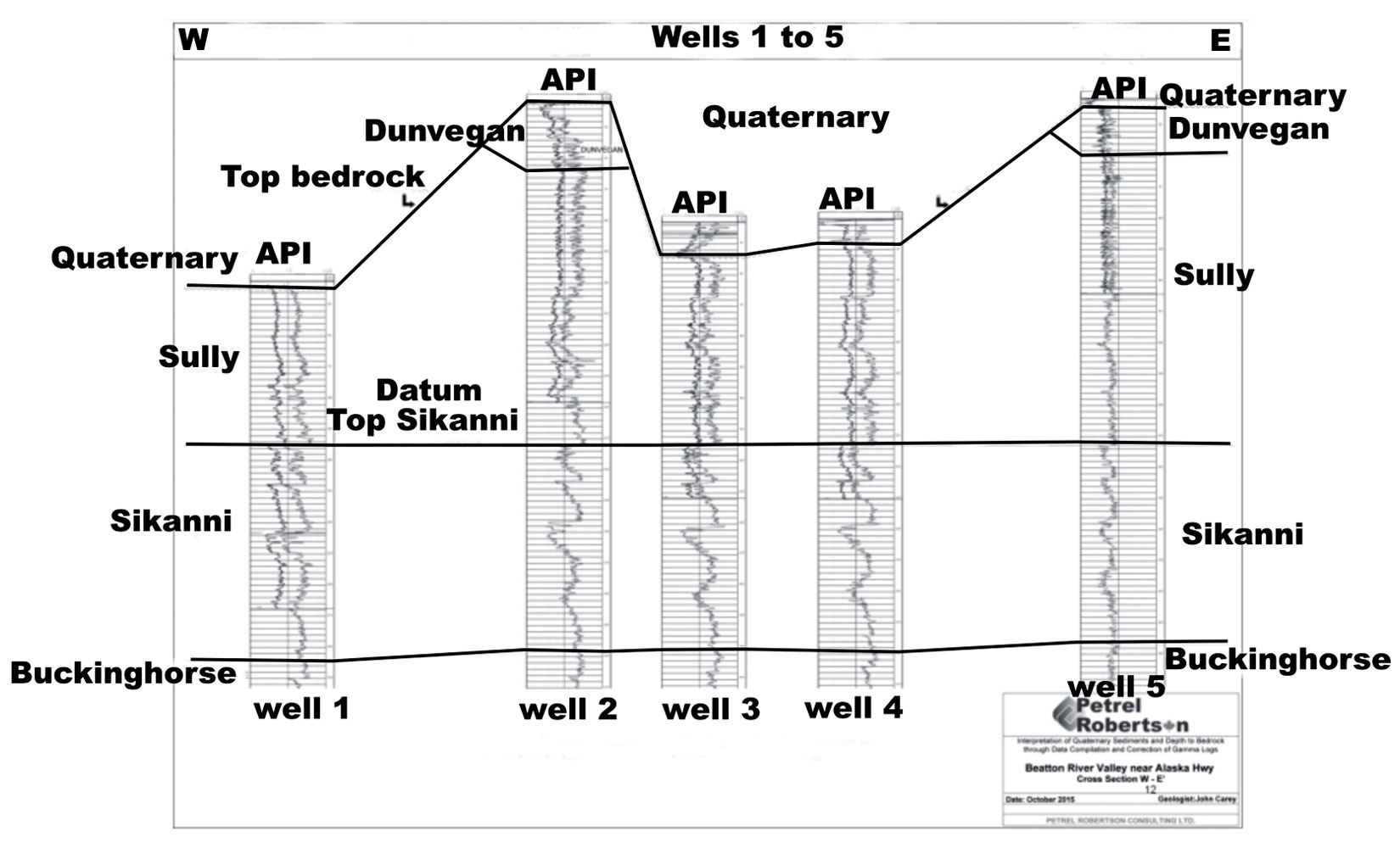
Figure 3 is an example of the gamma log interpretation for the SW corner of the main black block shown in Figure 1(a). Each well is colour coded with red being a petroleum well, blue being a water well, and yellow being a petroleum well with possible sand and gravel within the Quaternary section. Depth to bedrock (m) is provided as a number to the right of the well dot.
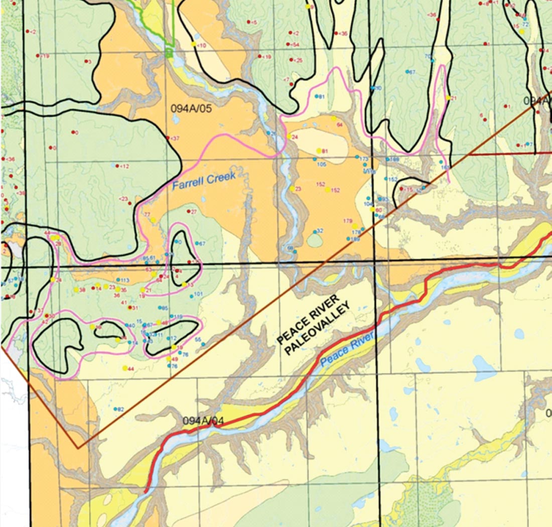
The well interpretation is overlain on a surficial geology map of the area (Petrel Robertson, 2015; Hayes et al., 2016) Light yellow represents glaciolacustrine sediments, orange represents glaciofluvial sediments, green represents glacial till sediments, and brown represents colluvial sediments. The black curves outline inferred paleovalleys and the red curves are the location of thick Quaternary fill.
Airborne EM data
The wells used for the gamma log study tend to cluster along the Montney play trend with just a few wells outside this trend (Figure 1(b). The gamma logs are therefore localized as well. The integration of these data with airborne EM data provides additional information between wells and within areas where there are few or no wells.
A 21,000 line km airborne electromagnetic (AEM) survey was flown using SkyTEM312FAST, a helicopter time-domain EM system. All traverse flight lines were flown in approximately a NE-SW direction 600 m apart, except for the Charlie Lake area which was flown E-W at the same spacing. Tie lines were flown perpendicular to the traverse lines at a spacing of 2400 m. Magnetic data were also recorded but are not discussed in this paper. The AEM system was towed beneath the helicopter at an average height of approximately 50 m terrain clearance. Technical details of the SkyTEMFAST system can be found in Brown et al., 2015 and in Brown and Efferso (in this issue of the RECORDER).
The in-line and vertical components of the time-varying magnetic field are recorded in approximately 30 time windows going from a few microseconds to tens of milliseconds. These data are used to produce quasi 2-D laterally constrained resistivity inversions (Auken et al., 2005). The final products are resistivity cross sections and depth slices over the entire survey area.
The inversions carried out by SkyTEM provide a quick look at the regional resistivity structure of the Peace project area. However their objective was to provide high quality EM data and not to provide a detailed interpretation of the data volume. In early 2016, Aarhus Geophysics Apps of Denmark was awarded a contract to reprocess and interpret 5 sub-areas, the Sikanni, Doig, Conoco, Charlie Lake, and Peace blocks (Figure 1(a)). The areas were selected based on the results of the gamma study, input from local communities, First Nations, and petroleum companies, and areas expected to have higher probability for locating aquifers (i.e. away from areas with shallow glacial till).
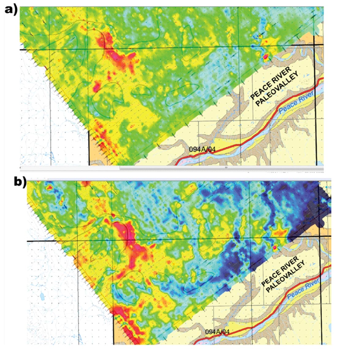
Aarhus Geophysics provided more detailed editing of the SkyTEMFAST data set to remove cultural effects and to correct for tree cover when estimating the height of the EM system above the ground. Preliminary inversions were carried out using quasi 2-D laterally constrained inversions (LCI). Preliminary LCI’s served the purpose of fine tuning the post-processing of the EM data, in terms of coupling and noise assessment. Final inversions were carried out using quasi 3-D spatially constrained inversions (SCI). In the SCI method the model parameters are tied together spatially with a spatially dependent covariance, which is scaled according to the distance between neighbouring stations. Where possible Aarhus compared the SCI inversions with the results of the gamma study for depth to bedrock, bedrock formation and Quaternary geology (Aarhus Geophysics 2016a, 2016b, 2016c, 2116d, 2016e). Figure 4 shows two resistivity depth slices produced by Aarhus in the SW corner of the SW Peace block shown in Figure 1(a).
Testing the geological interpretation
Well locations selected for testing
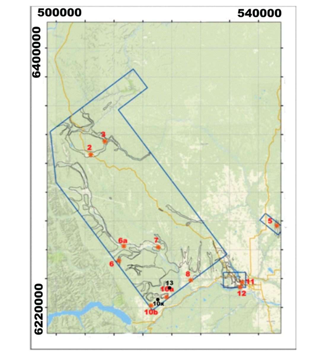
Well locations were selected for testing the geological model based on the interpretation of the gamma log and SkyTEM surveys (Geoscience BC 2016-18). The emphasis was on testing the geology, although finding water would be a bonus. Eleven sites were originally selected for testing the geological model (red dots in Figure 5). The majority of the wells (wells 6, 6a, 7, 8, 10a, 10b, 10x and 13) are in the SW quadrant of the main Peace block. Well 5 is in the Doig block and wells 11 and 12 are in the Charlie Lake block. Wells 2 and 3 are in the north block, south of the Sikanni River. Discussions with local stake holders and field examination of the areas selected resulted in several changes to these well locations.
| Well | Original easting | Original northing | Original line number | Final easting | Final nothing | Final line number | Approx. distance between original and final locations |
|---|---|---|---|---|---|---|---|
| Table 1. Original and final UTM locations for the 7 wells drilled and completed. The E-W flight line closest to the well is included for the original and final locations as well. | |||||||
| 3 | 533632 | 6335392 | L 104802 | 532800 | 6337068 | L 104503 | 1870 m |
| 6a | 546718 | 6262698 | L 115801 | 546650 | 6262600 | L 115801 | 120 m |
| 7 | 570600 | 6261960 | L 115801 | 570761 | 6262059 | L 118302 | 190 m |
| 10b | 565670 | 6221360 | L 123 202 | 564653 | 6220724 | L 123202 | 1170 m |
| 10 x | - | - | - | 570720 | 6225047 | L 123202 | - |
| 12 | 627284 | 6234107 | L 301701 | 627050 | 6234063 | L 301701 | 240 m |
| 13 | - | - | - | 579293 | 6234812 | L 122801 | - |
Eight wells were eventually drilled. Well 11 was drilled but the casing pulled after the drilling was completed. Table 1 lists the 7 wells that were drilled and cased. Five of the original wells shown in Figure 5 were drilled. Two additional wells were drilled; one for Simon Fraser University (well 13) and one for the University of British Columbia (well 10x). These were selected to meet specific requirements of these projects. Wells 6a, 7 and 12 were drilled at locations within 100 to 200 m of the positions shown in Figure 5. Well 3 was drilled approximately 1800 m from the original position and well 10b was drilled approximately 1100 m from its original position. Weatherford also ran a suite of petrophysical logs for all the wells in Table 1 except well 3.
For this paper, the Aarhus AEM inversions for wells 10b and 10x were selected for comparison with the geological log compiled by Quaternary Geosciences Inc., and the resistivity and gamma logs run by Weatherford.
Comparison of AEM inversions with geology and petrophysical logs
Well 10b
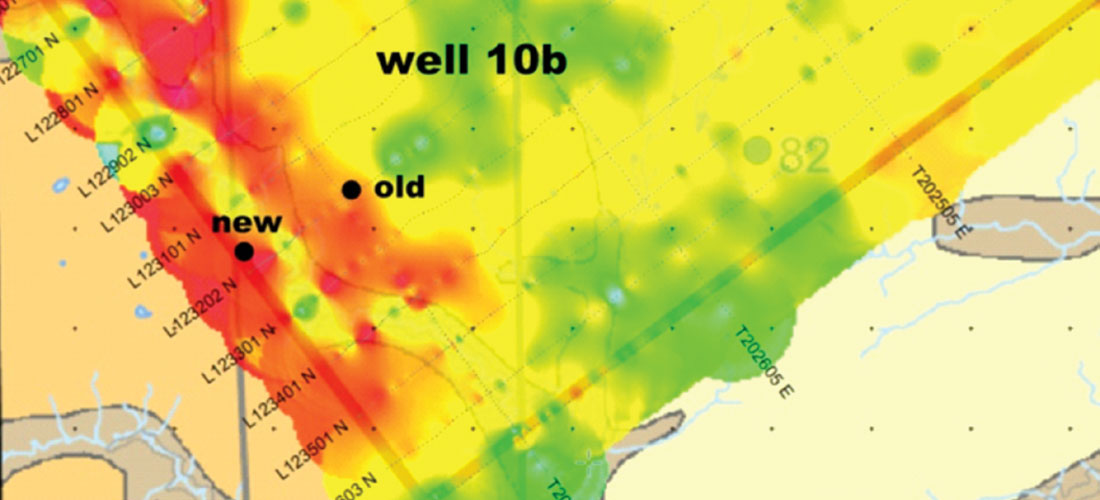
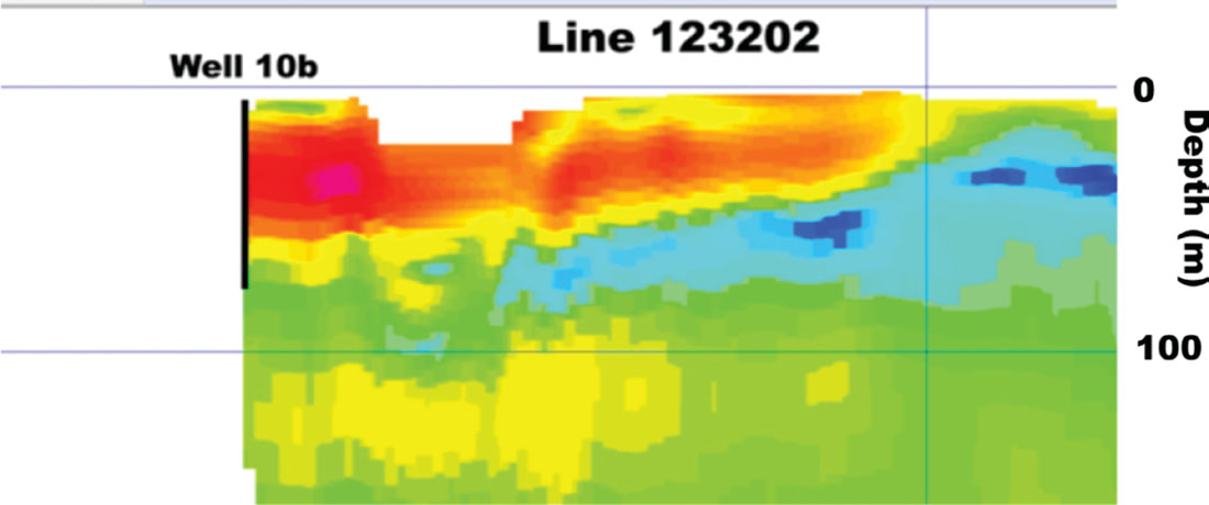
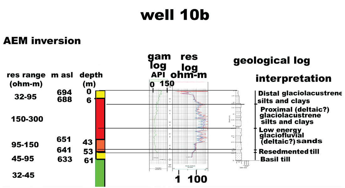
Well 10b is located east of Lynx Creek (Figure 6) . There are no petroleum or water wells close to this well. It was chosen because a well-developed glaciofluvial terrace is present in the area. A broad area of glaciofluvial sediments has also been mapped along the Lynx Creek drainage system. There is additional interest in the Quaternary section because recent landslides have occurred within the region. Figure 6 is a plot of the 15 – 20 m resistivity depth slice showing the original and actual well 10b location. Note well 10b has been moved nearly 1200 m to the west of its original location. Figure 7 is the Aarhus resistivity cross section for flight line 123202 showing the closest location to well 10b. Figure 8 is a plot of the interpretation of the AEM inversion at the well 10b location on line 123202 (on the left side) with the geological, gamma, and resistivity logs on the right side.
From 6 to 43 m depth the AEM inversion has resistivity values between 150-300 ohm-m, which is consistent with the resistivity values on the resistivity log. The Quaternary section within this interval consists of fine to medium sands with some silty sand beds. From 43 to 53 m depth the AEM inversion has resistivity values between 95-150 ohm-m, which is consistent with the resistivity log, although the depths are a few meters out. The geological section consists of very fine sand and sandy silt within this interval. The bottom zone of the resistivity log has values dropping rapidly as it goes into a zone of silty clay diamict. This is consistent with the AEM inversion which has resistivity values between 45-95 ohm-m.
Well 10x
Well 10x is located in a relatively high resistivity feature that is intermittent over a large region (Figure 9). It is located at the southeastern edge of the zone, at least on the 15-20 m resistivity depth slice. Figure 10 shows the location of well 10x on Line 123202, the closest flight line to the well. There is a high resistivity zone approximately 25 m thick which was the target of interest for UBC.
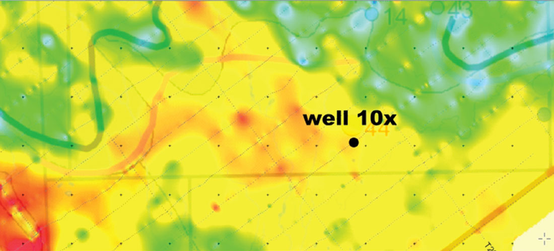
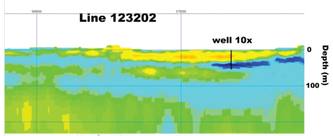
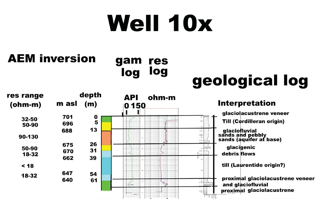
Figure 11 is a plot of the AEM inversion on the left with the resistivity, gamma and geological logs on the right. From 5 to 25 m the AEM inversion has resistivity values between 30-130 ohm-m. The resistivity log has an approximate value of 140 ohm-m over the same interval, while the geological log consists of silty diamict and fine to very fine sand. From 25 to 30 m depth the AEM inversion has resistivity values between 50-90 ohm-m. The resistivity log has values between 20-40 ohm-m. There is a wet pebbly fine sand that separates these two zones on the AEM inversion. Below approximately 30 m depth the geological section is mainly a silty clay diamict which is consistent with the resistivity values on the AEM inversion and resistivity log. The poorly sorted gravel bed observed near the base of the geological log (between 61 and 64 m depth) coincides with a resistivity high and gamma low (between 61 and 64 m depth but is too thin to be clearly seen by the AEM system.
Conclusions and future work
Airborne EM systems average over a significantly larger volume of material than the resistivity log, which only averages a few metres around the well bore. In addition, the resolution of AEM diminishes with depth due to averaging over larger volumes as the depth increases. Typical resolutions are a few m near the surface and around 10 m at depths of 60 to 70 m. The AEM system also requires a resistivity contrast of approximately 2.5:1 in order to resolve contacts, assuming the formations have appropriate thicknesses to be seen. The inversion process has resolution limits as well. The inversion process used by Aarhus Geophysics assumes the earth is at most two dimensional. However if three dimensional features are present then the inversion will produce incorrect results. In contrast, the resistivity log has a constant resolution of a few 10’s of centimeters independent of the depth. Metal casing near the surface of the well decreases the resistivity (i.e. increases the conductivity), so the resistivity log can be incorrect near the surface.
Keeping the above limitations in mind, the resistivity versus depth for the AEM inversions and the resistivity logs are in quite good agreement. This is the same for all the wells drilled except well 6a. Well 6a was problematic because there was no resistivity contrast between the gravels in the Quaternary overburden and the sandstone bedrock beneath the overburden. This is a situation that cannot be resolved by the airborne EM system. However the resistivity and gamma logs did show a subtle feature just above the sandstone. where there is a 2 – 3 m thick pebbly mud bed.
This study provides useful information on the relationship between the AEM inversions and geology. However the most important aspect of the project is to produce a hydrogeological model of the entire region. This will be partially addressed through a thesis being carried out at Simon Fraser University in the SW corner of the main Peace block (Aarhus Geophysics region 3) that will utilize all the collected data.


Join the Conversation
Interested in starting, or contributing to a conversation about an article or issue of the RECORDER? Join our CSEG LinkedIn Group.
Share This Article