Impact of Microseismic Location Uncertainties On Interpreted Fracture Geometries

Microseismic imaging of hydraulic fracturing is a growing technology throughout North America, and especially in the WCSB. Microearthquakes associated with hydraulic fracture stimulations are used to image the fracture network induced by the injection, and provide unique information about the fracture geometries. In an article in the March 2009 issue of RECORDER, I described the quantification of location uncertainties associated with individual microseisms. In this paper, the impact of these location uncertainties on the interpretation of fracture geometry is explored.

The position of the microseismic activity relative to the stimulated fracture network depends on the geomechanical deformation that results from the hydraulic fracture. The microseisms are generally considered to be mostly a shear deformation phenomenon, restricted to a tight zone around the hydraulic fracture network. To simplify discussion in this work, the microseismic distribution is assumed to be a direct map of the hydraulic fracture network. In some instances, however, this may result in an oversimplification: for example if the geomechanical deformation results in geometrical differences between the hydraulic stimulation and the microseisms. Nevertheless, it is worth noting that a common assumption made either implicitly or explicitly during interpretation of microseismic images, is that the microseismicity is a direct map of the stimulation.

This paper presents an investigation demonstrating how location uncertainties result in uncertainties in the interpretation of the underlying fracture network geometry. Synthetic computer modeling was used to artificially generate a microseismic dataset from an assumed fracture geometry, with locations perturbed according to assumed location uncertainty statistics. The synthetic dataset was used to illustrate how uncertainties in the fracture network geometry result from the microseismic location uncertainties. A new methodology to quantify the fracture geometry is also presented. A case study documents application of this methodology to two separate microseismic images of a hydraulic fracture stimulation. In one image, the microseismic locations were directly computed from arrival times and polarization individually for each event. The same data was then reprocessed using a technique to minimize the statistical errors in the arrival times, resulting in more accurate microseismic locations with smaller location uncertainties. In the context of this paper, it serves as a useful example to quantify the fracture geometry with two microseismic datasets, corresponding to a more-accurate and lessaccurate representation of the same fracture geometry.

Synthetic Data

A synthetic microseismic dataset of assumed locations was produced to examine certain aspects of the geometry of a microseismic ‘cloud’, in relation to the statistical perturbation of an underlying structure. Various components contribute to the location uncertainties in real microseismic data, and here we will make the assumption that the errors or uncertainties follow a normal distribution characterized by a certain standard deviation (σ). Thus, from a statistical population point of view there is a 68% probability of the location falling in a particular direction within one σ either side of the hypocenter or a 95% probability for it falling within two σ, defining a Gaussian probability density function (PDF). Also for the sake of simplicity, we assume that the error ellipsoid is spherical, meaning that the error is the same in all directions. For real data, nonlinearities in the calculation of the hypocenter result in nonlinearities and variations from a normal PDF (e.g., Maxwell, RECORDER March 2009). Specifically, nonlinearities associated with the velocity model can result in non-Gaussian PDF for the depth estimation associated with a horizontally layered velocity model. Nevertheless, the simplified location errors assumed here serve to illustrate several issues related to defining the underlying fracture geometry that results in a diffuse cloud of microseismic locations.

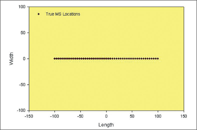
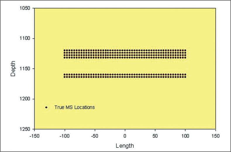
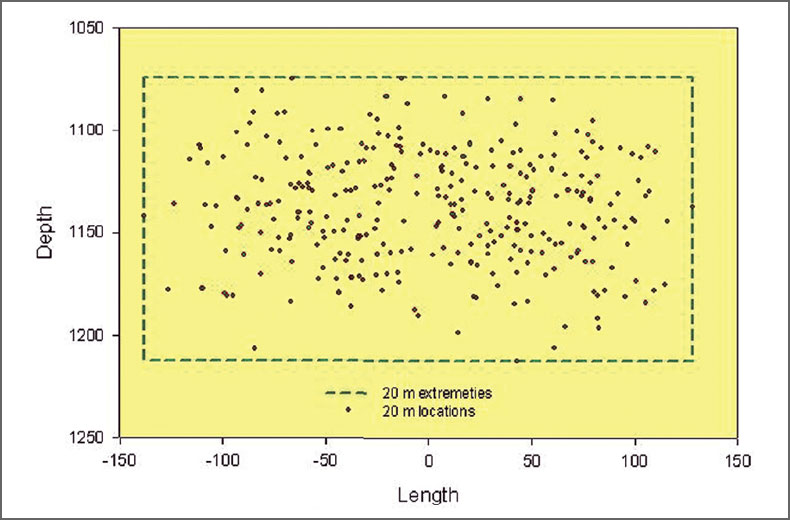
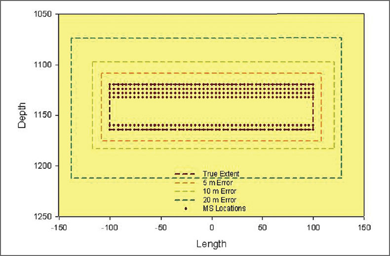
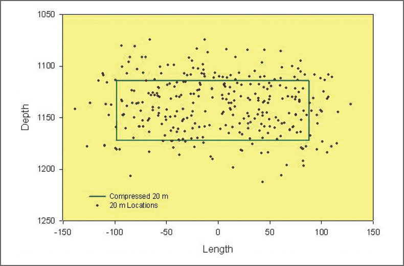
A geometric series of locations were assumed to define a ‘fracture’, confined to a vertical plane with microseismic ‘events’ spaced at 4 m along horizontal lines at discrete depths (Figs. 1 and 2). The horizontal distribution extends +/- 100 m at depths between 1120 m and 1164 m, with the exception of an interval between depths of 1132 and 1164 m where no events were assumed. These locations are referred to as the ‘true microseismic locations’ and have been constructed to loosely mimic the structure of the real dataset that is described later.

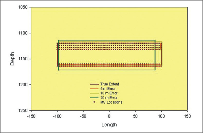
For the synthetic datasets, three different location error standard deviations were assumed: 5 m, 10 m and 20 m. For each error statistic, each true location was randomly perturbed in each of the Cartesian coordinates following a Gaussian distribution of the assumed statistics. Three different synthetic microseismic datasets or clouds were constructed as shown in Figs. 3 and 4. Obviously as the errors increase with the standard deviation, the extent of the microseisms also increases. The data with σ = 20 m is the most diffuse, containing events farthest from the true locations. For each event dataset, the extent of the microseismic cloud in specific directions (here referred to in the fracture sense of width, length and depth) can be defined from the extremities of the microseisms in that direction. Fig. 5 shows the extents relative to the dataset of σ = 20 m. Note that similar techniques have been used in the literature to measure the volume of the reservoir stimulated during hydraulic fracture treatments. It is useful to examine this measurement method in the context of the true locations and the true fracture extent. Fracture azimuth is not discussed here but could be readily estimated using a linear regression.

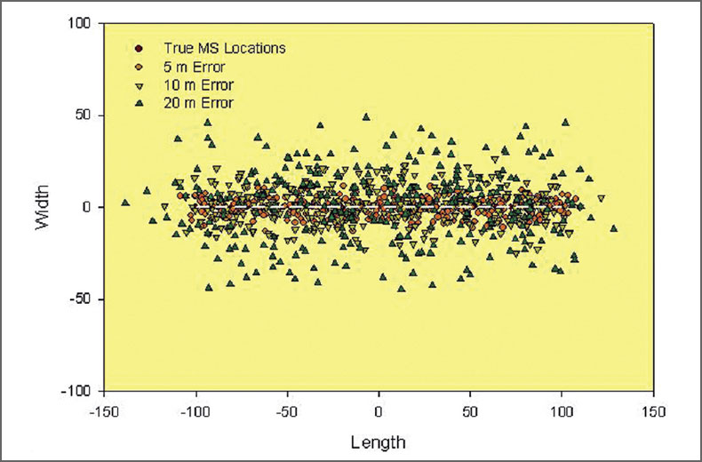
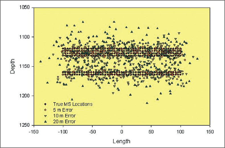
Fig. 5 shows a sectional view of the fracture extent based on a simple rectangle with sides defined by the extremities in the synthetic locations of σ = 20 m. The extents are defined by singleevent locations, and a more complicated shape could be defined to track the extremes of the microseismic cloud. This rectangle is a simple graphical representation of the fracture in terms of the distinct length, width and height. The corners of the rectangle are not meant to imply a fracture with sharp corners or any associated stress intensification. Fig. 6 shows a sectional view of the extremities from the three datasets, as well as the true extents and true event locations. This particular method of estimating the fracture has two significant limitations. First, the extent of the fracture increases away from the true fracture in all directions with increasing location error, such that more uncertain microseismic data would indicate a larger fracture or stimulated volume. Second, the fracture extent is overestimated regardless of the size of the location uncertainty. Clearly these are undesirable features of a monitoring technology when the stimulation objective is to maximize the stimulated volume. Although the degree of overestimation could be minimized to some extent by considering a smaller subset of the microseismic catalog, a better estimation is advantageous for a more accurate fracture estimation.

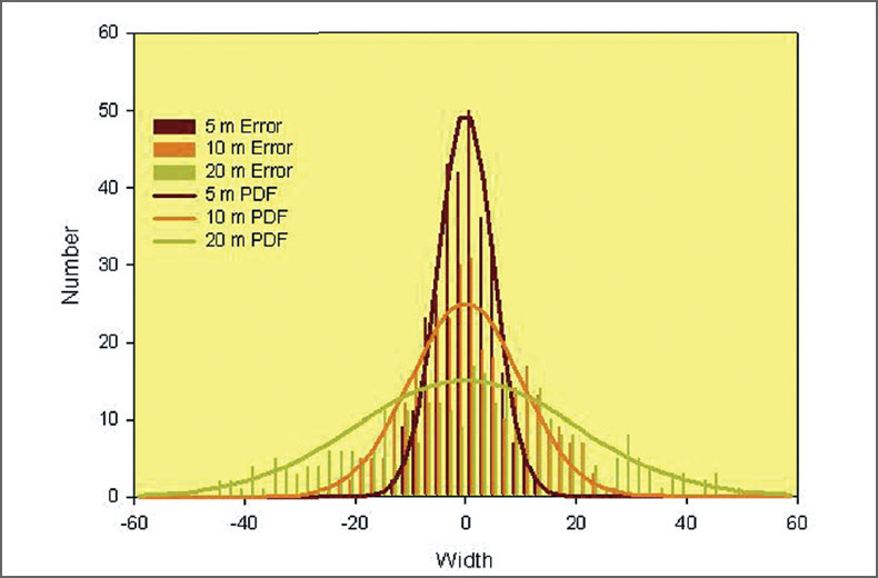
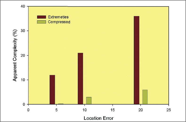
The synthetic data also illustrates two other potentially important factors that could lead to misinterpretation of a microseismic image. First, fracture complexity is sometimes measured from the microseismicity. In this example with a theoretical zero width fracture, the location uncertainties lead to apparent width of the seismic volume proportional to the location error (Fig. 7). By defining a simple fracture complexity measure as the microseismic cloud aspect ratio of the width to length ratio or percentage, the errors can lead to an erroneous indication of true fracture complexity. In this example the aspect ratio is zero, yet each of the clouds results in significant aspect ratios (Fig. 8) that increase with larger errors. As with the fracture volume, this is an undesirable feature of the monitoring because creating fracture complexity can be an objective of the stimulation.

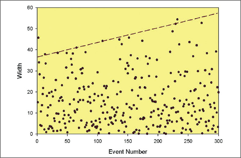
The second aspect of the location uncertainty, that could potentially be misinterpreted, is related to the temporal evolution of the extent of the microseismic cloud. Consider Fig. 9, which shows the width of the cloud (in this example for the 20 m error case) against the event number. With increasing size of the synthetic dataset, the observed width of the cloud increases. Since the fracture has zero width, this plot is simply showing the increased probability for outliers that deviate more from the mean of the PDF as the statistical population grows. Nevertheless, the increase in width could be falsely interpreted as temporal fracture growth.

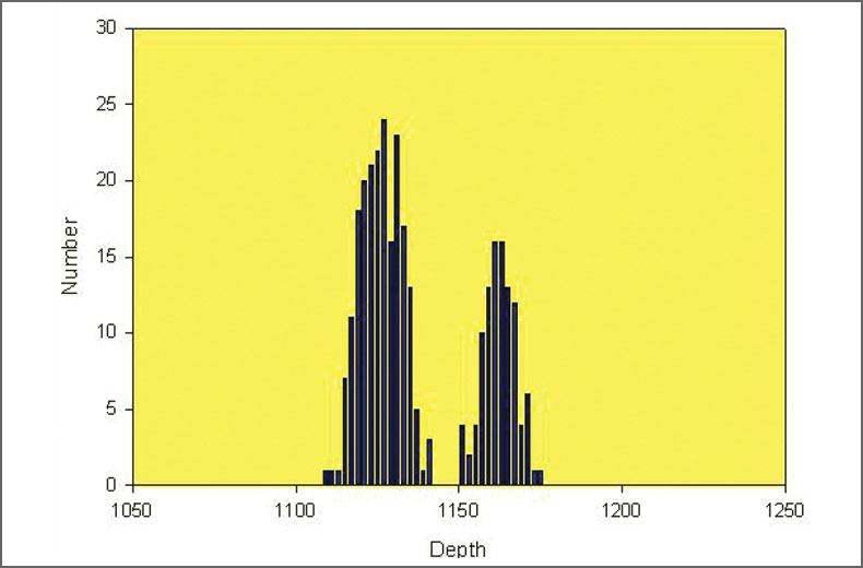
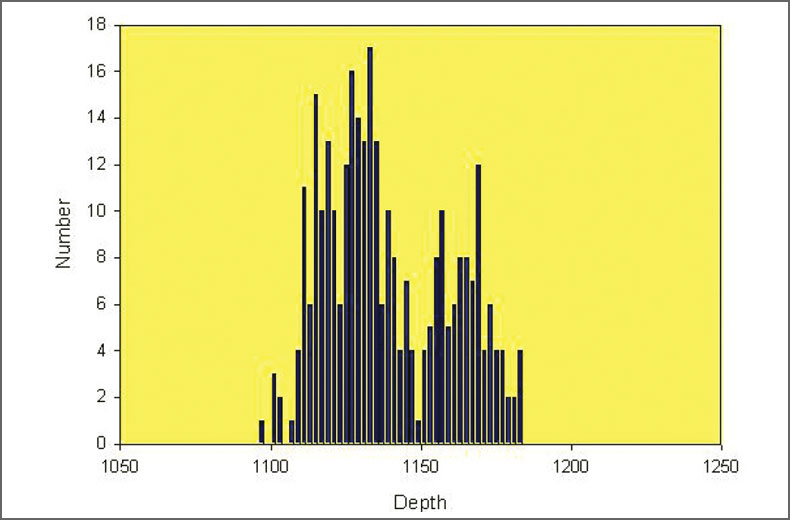
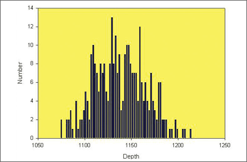
Another important aspect apparent with the synthetic data is the ability to resolve small features relative to the location error. Consider the depth distribution of the true locations, occurring between 1120 and 1132 m and 1160 to 1164 m. Figs. 10, 11 and 12 show depth histograms for the three location error datasets. For the 5 m error, clusters are easily seen for the two depth intervals. With the larger 10 m error, two separate clusters can still be seen but are blurring together. In the case of the 20 m error, the separate clusters can no longer be distinguished.

As indicated above, the use of the extremities of the microseismic cloud does not offer an accurate measure of the fracture geometry and can result in misinterpretation. To explore an alternative, consider the width histograms shown in Fig. 7. Also shown are the PDFs, which have been renormalized to the event density for each of the assumed errors. These PDFs can also be estimated by integrating the individual PDF for each of the perturbed event locations. The extremities of each cloud, as discussed previously, are at the tail ends of these PDFs. However, by considering the one-sided tail of the integrated PDFs of each cloud, a better estimate can be made of the average of the distribution. This value will be closer to the center of the microseismic cloud than the case of the extremity, so it will tend to reduce the estimate of the fracture dimension. We therefore define this as a ‘compressed’ estimator. Loosely, the method is conceptual similar to ‘collapsing’ techniques. The exception is that the individual event locations are not modified; rather, the data are used to model the cloud extension related to the location uncertainty. Several methods of estimating this average can be envisaged, although here a relatively simple method is used. Once the extremity in any dimension and the PDF are estimated, the events within 2σ are identified. The average standard deviation within that region could be computed to achieve a better estimate, but here we use just the uniform standard deviation of all the events. If the number of events in this 2σ window exceeds 95, there is a probability greater than 1 of the extreme event being beyond the 95% mark and therefore the search region from the extreme event is extended to 2.5σ. Within this search region the mode of the data distribution in the window is selected. An estimate of the mode uncertainty is taken as a one-sided standard error estimate 2σ/√N, where N is the total number of events. More sophisticated estimates of the average and one-sided PDF could be envisaged but have not been considered here.

In Fig. 13, the compressed fracture extent is shown for the case of σ = 20 m. Notice that in comparison to the previous extremity based method, the fracture extent is closer to the main part of the cloud, and within the sparsely populated edges. Fig. 14 shows the extents for all the data compared with the true event locations and true fracture extent. The agreement is fairly close to the true extents, especially for the most accurate dataset. Also shown is an attempt with the most accurate data to define the two subsets of the data, so that for σ = 5 m two separate rectangles are shown around the two clusters. The estimate for the 10 m error data also defined the two sub-clusters at the correct depth.

Based on this synthetic example, the compressed method of estimating the underlying structure is significantly more accurate compared with the method based on the extremities. Furthermore, the results are relatively independent of the magnitude of the error and are not biased towards either overestimating or underestimating the fracture extents. Fig. 8 shows the aspect ratio of these cases, which is significant reduced compared with the previous method. In fact, none of these aspect ratios would be a statistically significant complexity variation from the true value of zero. Clearly, the compressed method results in a superior estimate of the fracture extent.

Case Study

Microseismic imaging was performed on a multistage stimulation of a well in the Canyon Sands formation of West Texas. The case study has been published previously (Raymer et al., 2008 SEG in Las Vegas), and only a relatively few facts are repeated here. The Canyon sands in Sawyer field are Lower Wolfcampian in age. The sands were deposited as a series of deep water, slope-fan deposits in a wedge-shaped interval. These slope-fan deposits are highly variable in thickness and lie along and basinward of the southwest margin of the Eastern Shelf of the Permian Basin. Several depositional facies (e.g., conglomeratic sandstones, turbidites, hemipelagic mudstones) are combined to form the basic depositional elements of submarine fans. These elements display complex interbedding both laterally and vertically, thus leading to a very compartmentalized reservoir related to lateral porosity and permeability changes. Low permeability of these reservoirs requires hydraulic fracture stimulation to increase productivity of the producing sands. Six injection stages lasting about 30 min each were utilized to stimulate the six depth intervals ranging between 10 to 34 m in length. The well casing in these intervals was perforated and sealed off by packers from previously perforated intervals (starting from the deepest depth interval). In order to decrease loss of fluid due leak off the viscosity of the injected brine was increased by adding low concentration of polymer and CO₂. In the beginning of each stage, the injection rate was increased stepwise up to 100 L/s to result in a final wellhead pressure between 25 and 30 MPa. After more than 10 min of injection, proppant (grain size 0.6 mm) was added to the fracturing fluid to keep the hydraulic fracture open. The proppant concentration was gradually increased up to the final 1 kg/L. In each stage, more than 100 m3 of fracturing fluid and about 20 m3 of sand was placed into the reservoir formation. The data was recorded with an eight-level triaxial sensor array, with sensors vertical spaced at 30 m in an offset observation well. The observation well was located approximately 200 m from the treatment well.

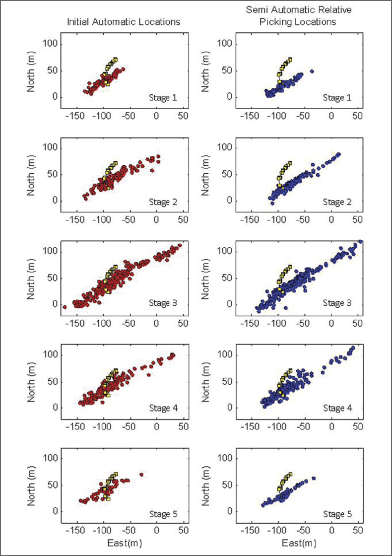
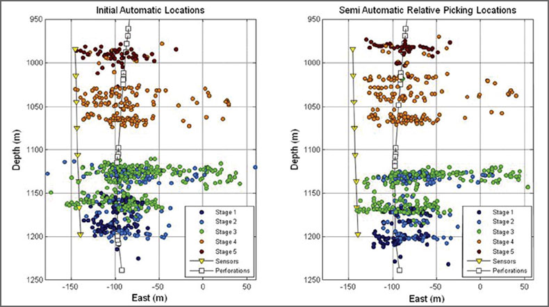
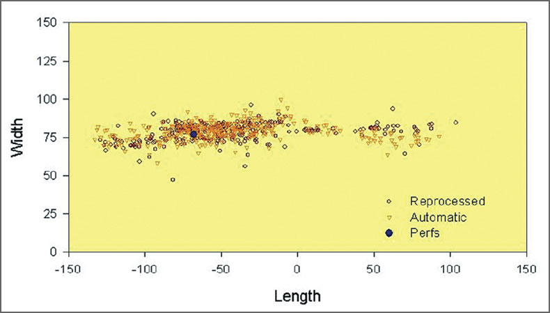
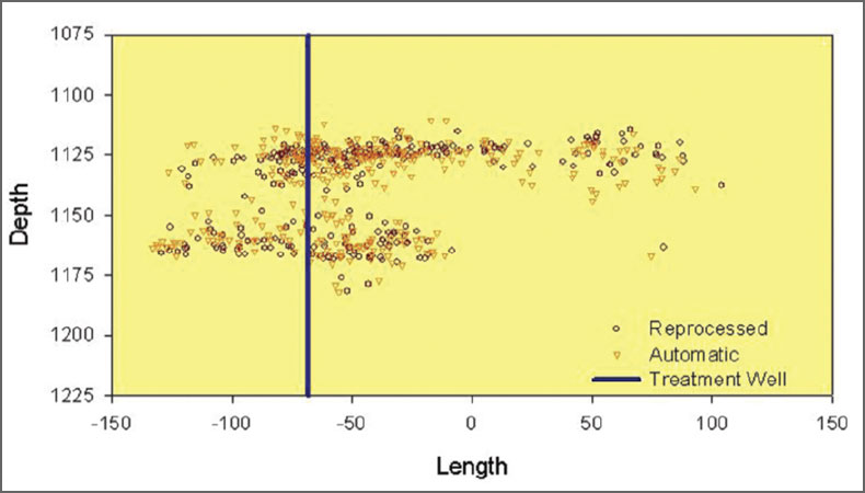
Original microseismic locations were computed automatically using a migration based algorithm. A subset of the data with high signal-to-noise ratio were selected and used to test a semiautomated relocation method. The technique makes use of signal similarity between events in order to ensure that the arrival time picks are consistent relative to aligned peaks and troughs in the seismic traces, decreasing the arrival time uncertainty and ultimately improving the location accuracy. The data was rotated into length and width directions to facilitate presentation here, and also the mean position of each dataset were equalized to account for a small offset between the two. Fig. 15 and 16 shows the original and improved locations.

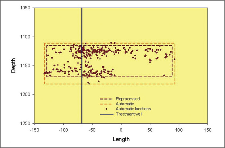
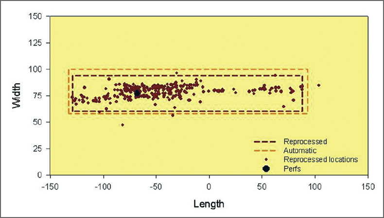
As before, the extremities of each dataset were first used to estimate the fracture extents, as shown in Figs. 17 and 18. Median estimates of the maximum length of the error ellipsoid were used as a uniform error estimate for all of the events in each dataset. These fracture extents are mutually consistent, although the extent of the reprocessed dataset is less than the automatic locations, presumably associated with the increased accuracy. A few obvious outliers were ignored for both the extremity and compression techniques. The results of the compression technique are shown in Figs. 19 and 20. The results are again mutually consistent within the location uncertainties, although the compressed fracture extent is smaller and more consistent with the highest density of microseismic events in the respective datasets. The one difference between the two datasets, although still statistically consistent, is in the width extent. The more accurate reprocessed dataset indicates significant fracture width, suggesting fracture complexity. The issue of the width and complexity is explored further in the following paragraphs.

The compressed fracture extents indicate statistically significant fracture width for the reprocessed data. Although the extents of the automatic and reprocessed locations are consistent with estimated errors, the reprocessed width is statistically significantly non-zero. Fig. 21 shows the aspect ratio of the microseismic cloud for both datasets with the extremity and compressed techniques. Clearly, the extremity technique indicates an artificially more complex structure. However, the compressed analysis of the reprocessed data is the only example that is statistically significantly non-zero. In the section view shown in Fig. 19, there are clearly two different depth clusters that also appear to have different extents. The compressed technique was further analyzed to assess the differences in the two clusters.

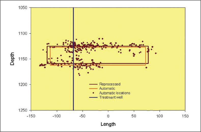
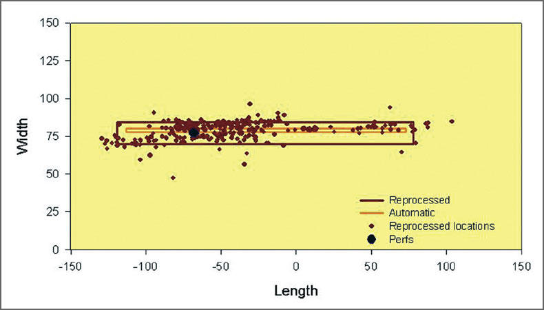
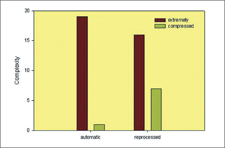
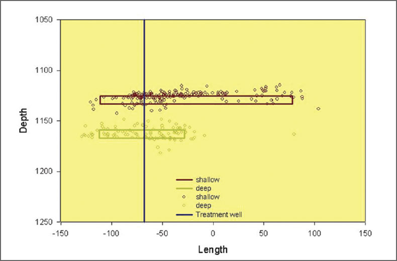
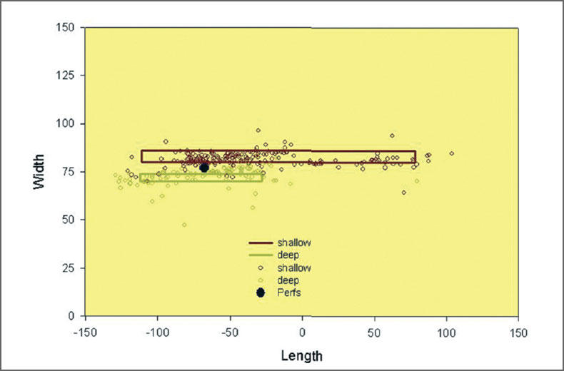
Fig. 22 shows a sectional view of the compressed extents after dividing the reprocessed data into two distinct datasets based on depth. For each, the compressed extent shows a substantial difference in the length of each cluster; the shallower cluster has a much larger length. The map view (Fig. 23) also shows that each cluster has a relatively narrow width, although the width of each cluster does not overlap. Therefore, the observed complexity in the overall fracture extent is simply due to a geometric offset between the shallow and deep clusters in terms of both depth and width. The width offset may be a result of the slight wellbore deviation, although the interaction between specific depth clusters for different stages of the stimulation of the well could also be related to the offset.

Conclusions

1. The locations of spatial extremities of the microseismic datasets are typically related to statistical outliers and controlled by the location uncertainties.
2. Fracture extents interpreted from the spatial extremities of the microseismic cloud are biased by the location uncertainty and tend to overestimate the extents proportionally to the average location error.
3. Even for simple fracture geometries, location uncertainties will result in a relatively wide microseismic cloud that could potentially be misinterpreted as a complex fracture.
4. The probability of statistical outliers at larger offsets increases and the number of events increases, which could be misinterpreted as dynamic fracture growth.
5. Using a technique called compression, the probability density function can be used to distinguish the spread of locations related to the location uncertainty from the fracture geometry.
6. The compression technique is less biased by the location errors, and it does not tend to overestimate the fracture extents.
7. The compressed fracture technique used to investigate the extent of a real dataset, produced similar results for two distinct images of the fracture: a preliminary and refined image with more accurate locations.
8. The fracture extents were found to be similar between the two images, validating the compression image.
9. The reprocessed locations indicated a fracture with a significantly non-zero width, although with further analysis the events were found to be two distinct depth clusters, each with a relative simple fracture without significant width.