Hydraulic Fracturing Data Integration – What Should I Be Asking My Engineer and What Are They Trying to Tell Me?

Communication between technical disciplines in the oil and gas industry is always a challenge. Different definitions, varied nomenclature, diverse cultures and backgrounds all make for challenges when working in the multidisciplinary world of petroleum extraction. This paper is an abridged version of the November 2016 Keynote Luncheon Presentation entitled “Integrating Data – How Geophysicists and Engineers Can Work Together to Improve Hydraulic Fracturing” and focuses on the basic reasons for hydraulic fracturing and what the engineers’ goals generally are when developing a hydraulic fracturing treatment design. Opportunities for potential areas of data integration between the engineering and geophysical world are provided, and the paper concludes with some questions that might help to spur better communication between these two disciplines.

Introduction

According to the Merriam-Webster dictionary, “communication” is defined as “the act or process of using words, sounds, signs, or behaviors to express or exchange information or to express your ideas, thoughts, feelings, etc., to someone else”. One of the biggest concerns with multidisciplinary integration in the oil and gas industry is basic communication. How do different disciplines look at techniques or applications? How do they approach them? What’s important to each person involved?

When discussing how geophysicists and engineers can work together to improve hydraulic fracturing, it is probably best to start with a discussion of how engineers look at hydraulic fracturing. Hydraulic fracturing is known as a stimulation technique. In essence, it allows the well to produce more than it ever could have under natural, non-damaged conditions. By definition, stimulation means that a well exhibits a negative skin factor, S. If damaged, the skin factor will be a positive value. These impacts can be seen when placed into Darcy’s radial flow equation, Eq. 1, where a positive skin factor drives down the flow rate, Q.

Q = flow rate
k = permeability
h = height
P_i = initial reservoir pressure
P_wf = well pressure
B = formation volume factor
μ = viscosity
r_e/r_w = ratio of drainage radius to wellbore radius
S = skin factor

Another way to look at a hydraulic fracturing treatment is that a negative skin factor makes the wellbore radius, rw, “look” bigger to the reservoir, thus creating a larger exposed surface area and therefore increased flow rate. This impact can be observed in Eq. 2, where rwa is the “effective wellbore diameter”.

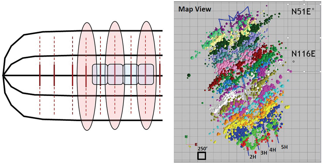
This effective wellbore diameter leads to a discussion of “effective length”. A hydraulic fracture’s length is a point of constant discussion, however, a major communication issue can be just which “length” is being discussed – there are actually four. The length of the fracture contributing to production, as described in Eq. 2, is the “effective length”. This is the most important of the three, since it is what contributes directly to enhanced production and reserve recovery. The other three are as follow: “microseismic length” is a measure of the distance from a wellbore at which microseismic events are detected; “hydraulic” or “pressurized length” is the distance to which pressure is transmitted from the treated wellbore during pumping; and “propped length” is the distance to which proppant is transmitted out into the reservoir. Although the latter two have an impact on the ultimate effective length, there is no direct link or percentage calculation. The resultant effective length is greatly impacted by such things as multi-phase flow, reservoir permeability and pressure, well spacing, and treatment design. Figure 1 demonstrates these various definitions of length.

Coupled closely to effective length is fracture conductivity, which is defined as the permeability of the fracture multiplied times the width of the fracture. Adequate fracture conductivity given a reservoir’s producing capacity helps to establish the maximum effective length for a certain well-reservoir system. These concepts apply to all reservoir systems, however, the focus of this article will be on unconventional reservoirs with horizontal wells that are treated with multistage hydraulic fracturing treatments.

Goals of Hydraulic Fracturing

When designing a hydraulic fracturing treatment, there are usually several goals that are attempted to be accomplished. The importance or ranking of these goals will vary depending on the specific objectives of the company or engineer that is designing the treatment. Along these same lines, the data that is needed to improve or aid the design (and the associated cost to acquire them) is also a function of the overall treatment goals.

In general, maximizing the effective fracture length is a major objective for most treatments. Quite simply, the longer the effective fracture length, the larger the drainage area for that well, and the fewer wells needed for a given area. Coupled with the effective length is the desire to achieve adequate fracture conductivity for the available reservoir deliverability. Minimizing the potential damage through gel damage, crushing, filter cake build-up, etc. to the established conductivity is also desired. As with the damage to the fracture conductivity, minimization of damage to the formation itself should be pursued.

In multistage treatments, such as those pumped in most horizontal shale wells, maximizing the number of zones producing and draining everything that is connected to the well should be a focus. It is frequently reported that the number of contributing stages is well below the number actually pumped in many horizontal wells (<50%), which is obviously a large waste of resources under such circumstances. Also, when considering the number of stages and other variables for a given well, the importance of acceleration or addition of reserves needs to be understood. Both can be achieved but are not directly related. (Barree et al. 2015). Pursuit of acceleration, without adding reserves, can destroy economic value.

Finally, it might be obvious, but still needs to be stated, minimization of treatment costs is always a desire. However, costs need to be considered under the other goal conditions, and perhaps maximizing net present value is a better way to consider these systems. Overall, it is impossible to maximize all of the goals, therefore, the engineer must focus on what is most important to them and their management and design accordingly.

Scale

Like many areas in the oil and gas industry, the scale of various measurements needs to be taken into account when considering hydraulic fractures. Bedding planes or mechanical property variations on the order of 1-2 cm can impact fracture growth, especially in the vertical direction. Such a small scale is obviously below the resolution of many data-gathering techniques and this fact needs to be considered when integration of data sources is attempted.

Potential Opportunities for Integration

There are several places that geophysicists and engineers can work together on data integration for improved hydraulic fracturing, not all of which can be discussed in the space of this article. Focus is therefore placed on three of the more obvious and perhaps easiest areas where integration can be performed, while having a significant impact on treatment design and overall field development and characterization: 1) diagnostic fracture injection tests (DFIT’s); 2) fiber optic measurements; and 3) fracture modelling.

DFIT’s

DFIT’s have become popular in unconventional reservoir development as they provide information about a number of reservoir characteristics including fracture pressure, closure pressure, process zone stress (the difference between fracture and closure pressures), leakoff mechanisms including the presence of natural fractures, reservoir pressure, and reservoir permeability. This article focuses on the application of these results and not the actual tests themselves, therefore, for further information on such, the reader is referred to Barree et al. 2009, Barree et al. 2014, and Barree and Miskimins, 2016.

DFIT’s are frequently used to help calibrate calculated closure pressure (minimum in-situ stress) logs. While one DFIT in the zone of interest can provide information regarding that zone, multiple DFIT’s taken in a vertical profile can provide critical information about stress changes and how they may or may not impact height growth. This is the same with process zone stress values, which can also have a significant impact on fracture containment in the vertical profile.

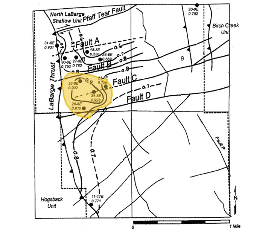
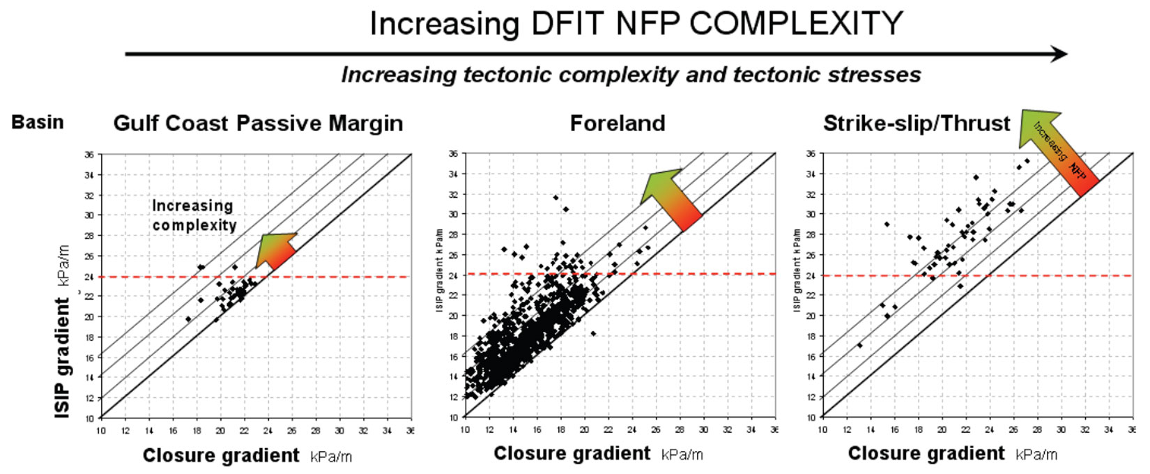
In addition to calibration of vertical stresses, this type of information can also be plotted across a play or basin and linked to other data. Figure 2 shows a small field where DFIT data results corresponded to 3D seismic information, whereas Figure 3 shows DFIT values associated with structural complexity across an entire basin. Other DFIT results, such as pore pressure and permeability can also similarly be plotted in vertical and plan views.

Fiber Optics

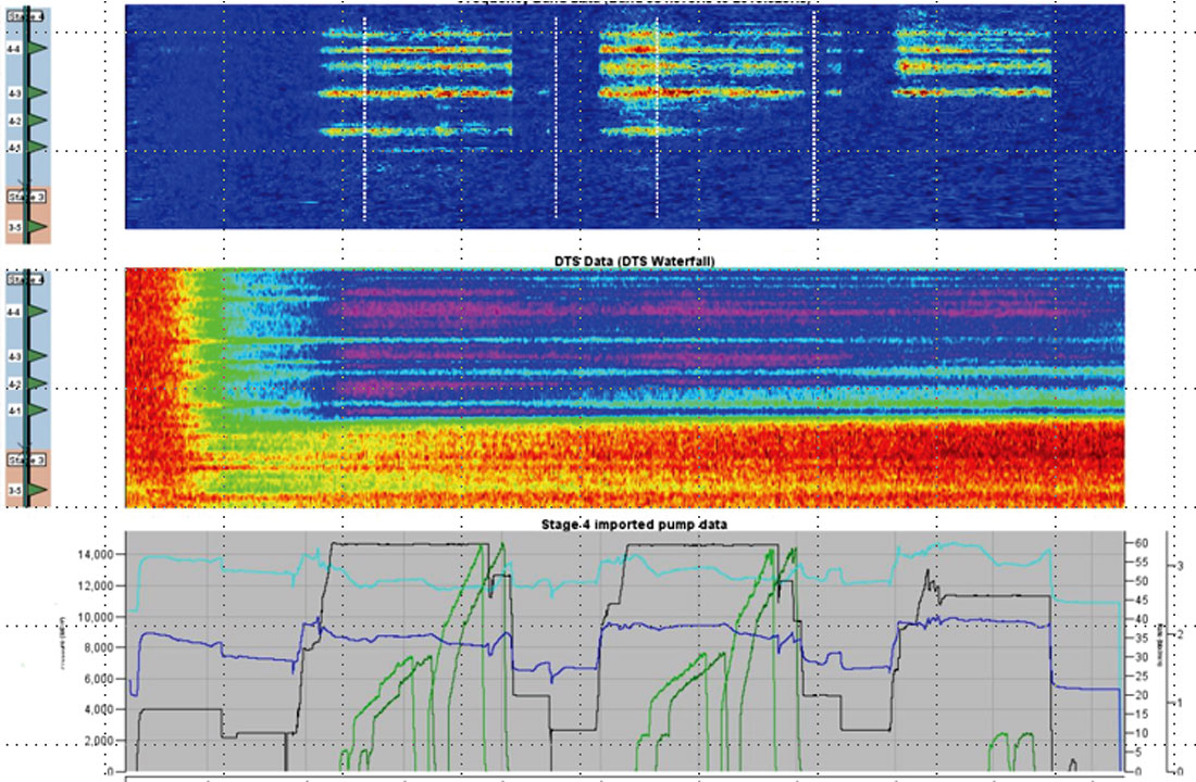
A relatively new area for integration is the use of fiber optics including distributed acoustic and temperature sensing (DAS/DTS). This type of data is providing detailed, dynamic information on what is occurring downhole during multistage fracturing treatments, as well as during post-treatment production. Figure 4 shows an example of perforation cluster response to diverter drops during a treatment stage, as well as behaviour during the rest of the treatment. This type of data is also providing information on leaking bridge plugs, inter-stage communication, and zones/clusters turning on and off during production.

Fracture Modeling

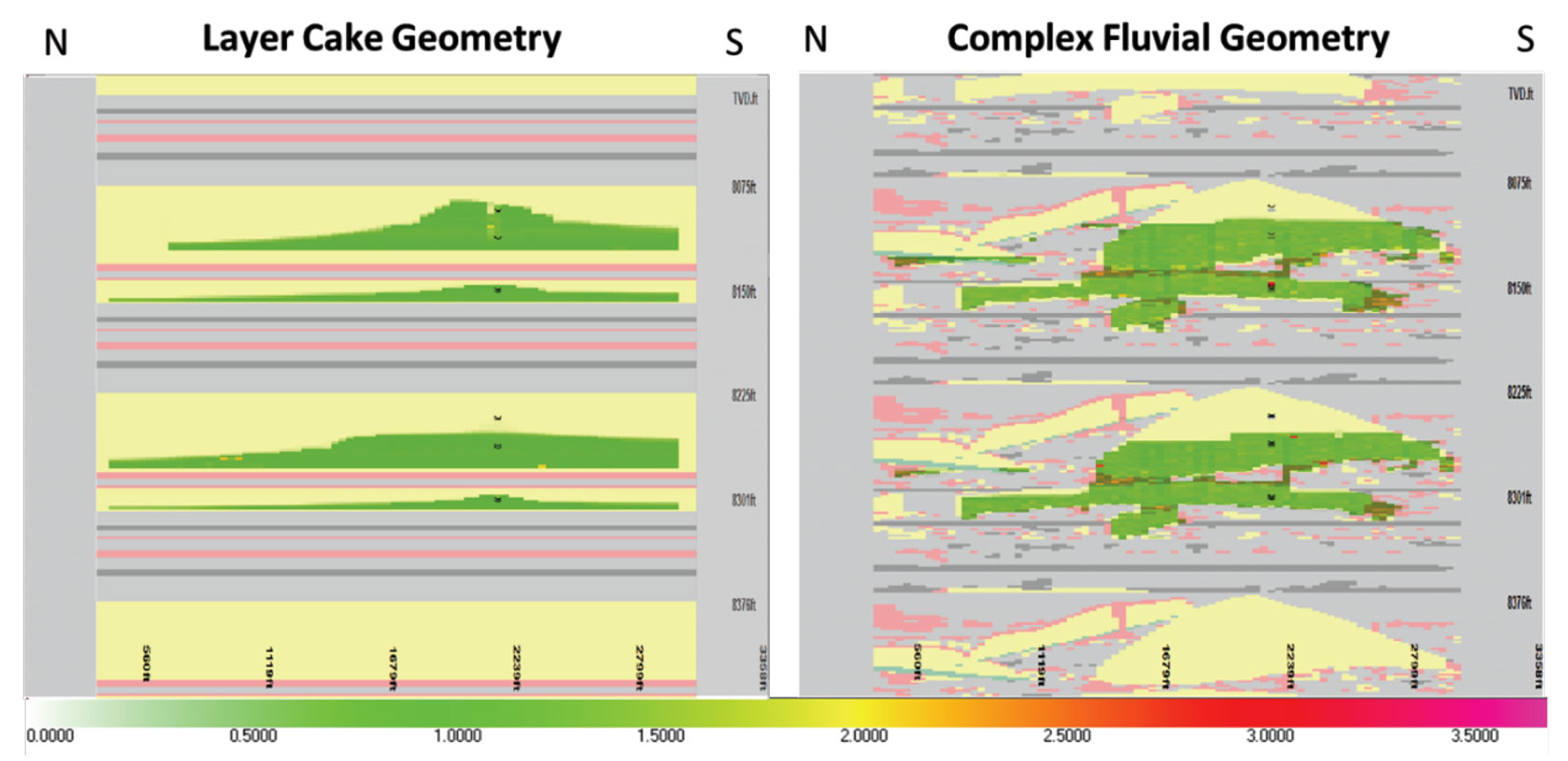
Modelling of hydraulic fractures is another area where engineers, geophysicists, and geologists can work together to improve our understanding of fracture behaviour. Helping to construct an accurate depiction of the geologic setting, in both a vertical and lateral setting can greatly improve the results and credibility of fracture models. Figure 5 shows an example of such an improvement in a stacked, fluvial system and the significant impacts it can have on the model results when a detailed geologic system is incorporated. Especially for systems that have known geologic changes in a lateral direction, whether structural or stratigraphic, this will result in an improvement over a “layered cake” approach.

Another modelling area that needs to be addressed from a variety of perspectives is the stress field orientation and the fracture profile in relation to it. The present-day stress field has a clear impact on drainage pattern and fracture-well alignment. Additionally, the stress field can have a large influence on overall treatment efficiency, breakdown pressures, and the extent of longitudinal versus transverse fracture growth. Any insights into both large and small scale stress behaviours can be helpful on a variety of levels.

Conclusions

This article (and associated presentation) is not intended to be a comprehensive discussion of data integration between disciplines, but rather, it hopes to spur conversations between individuals to improve the efficiency and economic value of hydraulic fracturing. With that in mind, a few final questions are provided to help instigate these dialogs and perhaps facilitate that communication.

What should I be asking my engineer?

• How do you define “stimulated reservoir volume?” Is it the “effective stimulated volume” or something else?
• Can I provide you with some help from a structural standpoint for your model? Fracture swarms? Fault locations?
• Can your model handle structural components? Are they important to the fracture behaviour? If so, should we be looking at a way to handle them?
• Can I help you define sedimentary bodies? Terminations of such? Their mechanical properties?

What is my engineer trying to tell me?

• In unconventional reservoirs, longer term production data is usually needed before I can calculate drainage area.
• I really, really, really need to understand the 3D pore pressure distribution – can you help me with that?
• Initial completions can be inefficient; can you help me determine gaps (4D, fiber)?
• A “successful” fracturing treatment is not always an economically optimized fracturing treatment.

Hopefully, these thoughts will help improve your completions and spur some lively discussions!

Acknowledgements

The author would like to thank the editors of this special journal edition for the opportunity to contribute to it. Also, thanks to the DoodleTrain organizing committee for the initial opportunity to present these thoughts during their annual luncheon.