Depth Imaging – Above and Beyond Reflections: The Why and How of Your Pre-stack Depth Migration Project

Introduction

When I was a student, I learned the magical, melodic word “migration” but not in relation to butterflies, birds or wildebeests. Since then, I have dedicated several years of my post-graduate research work to migration, only to understand the brilliance of the Socratic Paradox that, "I know that I know nothing”. Several decades of pre-stack depth migration (PSDM) projects, and few mistakes later, I still have to admit that I do not know everything about depth imaging or PSDM, but I know more. My co-author, Mike Hall, and I are happy to share this knowledge, as well as the accumulated knowledge of our colleagues, in this article.

Depth Imaging - Above and Beyond Reflections. The title itself reflects how complex, non-stationary, and multi-layered the topic of depth imaging is. It certainly goes beyond reflections, both in imaging, as well as in some philosophical sense.

Why do we even do depth imaging? Would it be practical to ask of someone to spend so much extra time, resources, and money to commission the PSDM work including the associated and complex interval velocity model building? We are told that time migration can be used to solve certain imaging problems, but more complex ones, such as sharp lateral velocity changes, need depth migration. Where do we draw the boundary in the decision between time and depth migration?

• What are the practical aspects of a PSDM project? Where do we start?
• How do we gather the data and which data do we have to gather, anyway?
• Should I involve the interpreters at the onset, or do I need a petrophysicist?
• What about a geologist?
• How can I use my well information in PSDM, and do I even need it for all my projects?
• Can I do without it?
• How should I test for migration parameters?
• How should I set up the migration grid? And what about raytracing?

We will review these questions in the introductory section, and also later on, while discussing the practical aspects of PSDM project execution.

Further questions include, how can I handle anisotropy ambiguity, and what about the near-surface? What are these diffractions, anyways, and why are they so important? And, of course, the never-ending saga of velocity updating: where do I begin, what is my initial velocity model, how do I make it? Which update methods should I choose? Do I need tomography? How can I use my horizons and well tops? What are the rules, anyway, and are there even rules at all? We will try to answer these, and many other questions of practical PSDM project execution. We will also try to touch on selected project management aspects and cover such important topics as quality control and results presentation.

The last and the most important set of questions: Where do we draw the line and pronounce the project and efforts complete and satisfactory? Will it ever be satisfactory? What about interpreters and clients - how can we keep them content and happy? What will happen next, to the data and results, once I pass them on to the interpreter or QI group? How can we feel confident and good about the thorough and intelligent work we have done, while there are so many controversial opinions about the results and the methods themselves?

In this paper, we will try to tackle perhaps not all, but the majority of these questions, and will try to enlighten you and provide you with practical tools and approaches that are the result of our combined experience from several decades of onshore and offshore depth imaging work.

PSDM will still be an enigma, as complex and ever evolving as it ever has been, and likely will be for some time to come … but hopefully it will be a bit easier to handle and a bit lighter to approach.

“I know that I know nothing”
“ipse se nihil scire id unum sciat”
"I neither know nor think that I know"

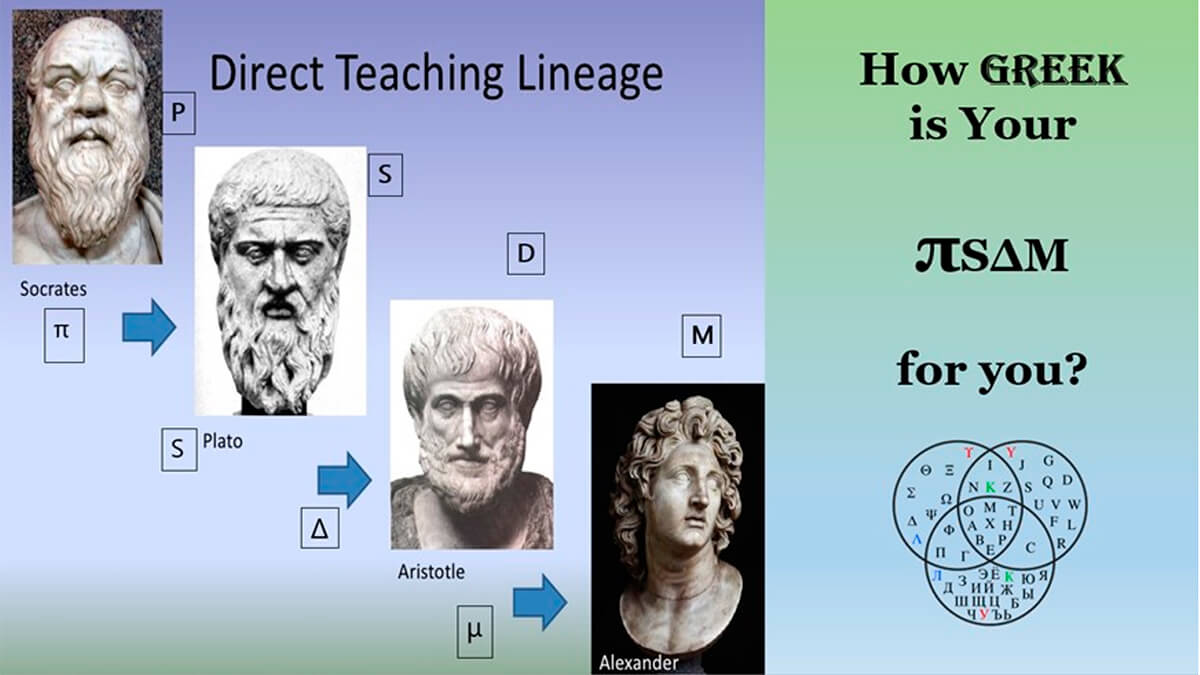
As mentioned, these phrases belong to the Ancient Greek (Athenian) philosopher, Socrates (Fig. 1). They are various permutations of a famous philosophical phrase called “the Socratic Paradox”. This phrase has been translated and interpreted by many different sources and presented in many diferent ways.

“I am wiser than this man, for neither of us appears to know anything great and good; but he fancies he knows something, although he knows nothing; whereas I, as I do not know anything, so I do not fancy I do. In this trifling particular, then, I appear to be wiser than he, because I do not fancy, I know what I do not know.”

Similar to these versions of one idea, one phrase even, people and industry have various approaches, points of view, and understandings of what is important in depth imaging. The good news is that, as in Socrates’ case, the knowledge is not stale but dynamic, and evolves and adjusts itself through intelligent, thoughtful processes, experience, and collaboration.

By the way, an interesting fact is that the enigmatic figure Socrates (as enigmatic as our beloved PSDM, probably), left no writings of his own. It was his students, such as Plato, who would write his words down for future generations (Fig. 2).

Luckily for us, we can capture and present our experiences without any difficulties, and can share them within the professional community, for example, through such excellent sources as the CSEG RECORDER.

But enough philosophy. Let us move to more practical matters.

Why Do We Need to Do Depth Imaging?

The most important question that depth imagers should be able to answer for their clients, for their peers, for their management team, but most importantly, for themselves, is: Why do we need to do depth imaging? There are many good reasons. We will highlight a few main ones here:

• Depth migration is a crucial step in addressing small scale velocity heterogeneities.
• Heterogeneities in the overburden cannot be accurately resolved through PSTM work alone. These small-scale velocity heterogeneities in the overburden can affect AVAz and VVAz analysis in shale plays (Goodway et al., 2016).
• Depth migration obliges us to build and incorporate an accurate geologically based near-surface interval velocity model, which is vital for correct PSDM imaging.
• Depth imaging enables us to obtain the highest structural and stratigraphic resolution.
• Anisotropy, a very complex and non-trivial component of the imaging, can only be properly handled within the depth imaging environment. This is expanded in the section on anisotropy.
• The method of converting PSTM volumes to depth that is used as an argument against PSDM work, often yields inaccurate and insufficient results due to the velocity model limitations which lead to problems in, for instance, achieving a primary geologic and engineering goal of staying in zone when drilling. A good PSDM result will have an accurate interval velocity model from the surface to the target and likely beyond. PSTMs that use RMS or NMO velocities, that are primarily only sensitive to vertical changes, cannot achieve such accuracy nor the shallow to deep integrity available from PSDM.
• Depth migration has a much higher chance of getting all the faults and fractures in the section positioned accurately, both laterally and vertically.
• With the recent advances in hardware capacity and computational speed, depth imaging should become a standard practice.

Based on the previous statement, there could be raised a fair question: Do we even need to do PSTM anymore? The answer is yes, of course, in fact it is difficult to achieve a good PSDM result without well prepared time processed data. In addition, time volumes are often used as guidance and as a reference point for the follow up PSDM results.

Input Data Considerations

The input to PSDM should be properly QCed. The accurate and thorough depth imager should never skip this step. I’m listing some of my favorite culprits here, but it does not mean there are no others:

• Geometry consistency
• Grid accuracy
• Acquisition and coordinate systems conversion pitfalls
• Time processing caveats that affect PSDM result
• Diffraction preservation in pre-processing
• Initial velocity work (“bullseyes” and vertical picking imprint issues)
• Near-surface model plausibility
• Residual statics: unwelcome anomalies and/or excessive smoothing
• Poorly handled noise attenuation (can destroy steeply dipping signal).

Look for anything your eye, experience and heart can detect. Be vigilant but not afraid… not afraid to ask questions and not afraid to question.

Figure 3 illustrates several potential problems that can affect future PSDM work. To avoid inconsistent or erroneous grids, survey corner points can be checked against the navigation or acquisition maps.

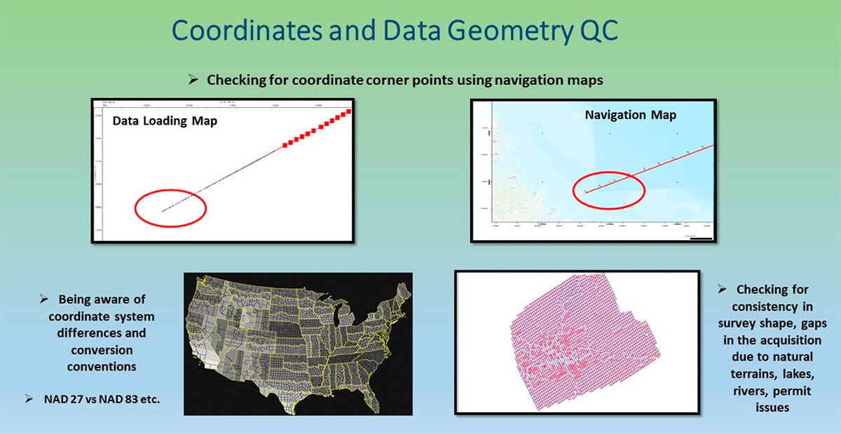
Various holes in the acquisition should only be accepted by you when it is verified that they are a result of naturally occurring terrains, lakes, rivers, permit related skips, etc. This will prevent processing of an incomplete dataset or half of the loaded area. Where gaps in acquisition occur, as is often the case with land data, a regularization procedure, preferably in 5 dimensions (5D) can improve the migration, lessening migration artefacts (smiles) and yielding more accurate amplitude information as required by any ongoing QI work. This process, whilst generally effective, is not a substitute for well sampled data acquisition in the first place.

It is important to know the data coordinate systems and proper conversions well. For example, data from the USA might come in a Plane State Control System and not UTM, as expected by most algorithms and software.

The time processing prior to PSDM should be thorough and preferably PSDM tailored and performed with future PSDM objectives in mind. (See later section on PSDM.)

Figures 4 to 7 are examples of some real-life scenarios of importance for accurate time processing prior to successful PSDM work.

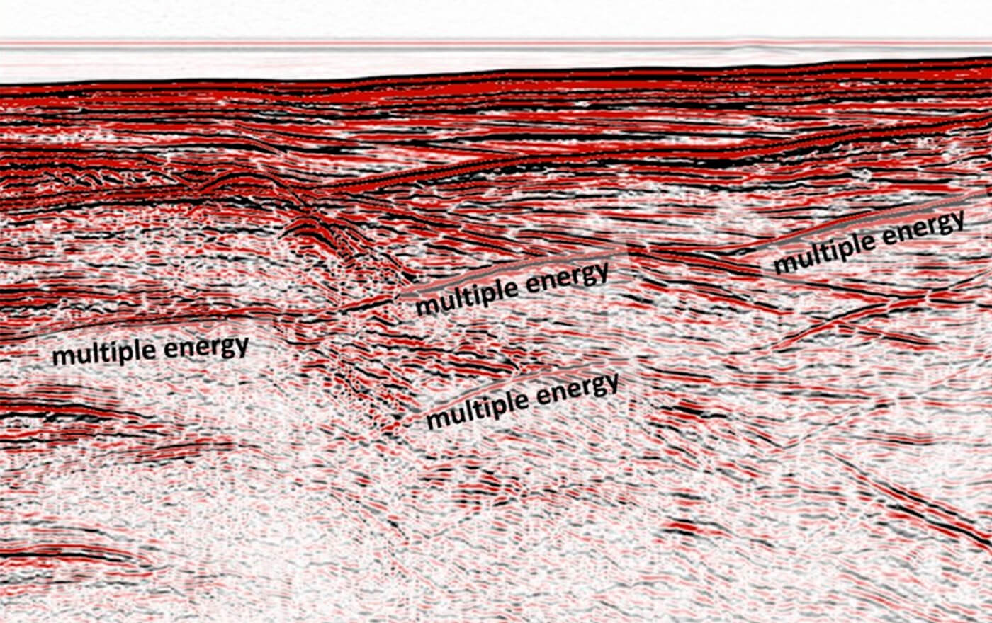
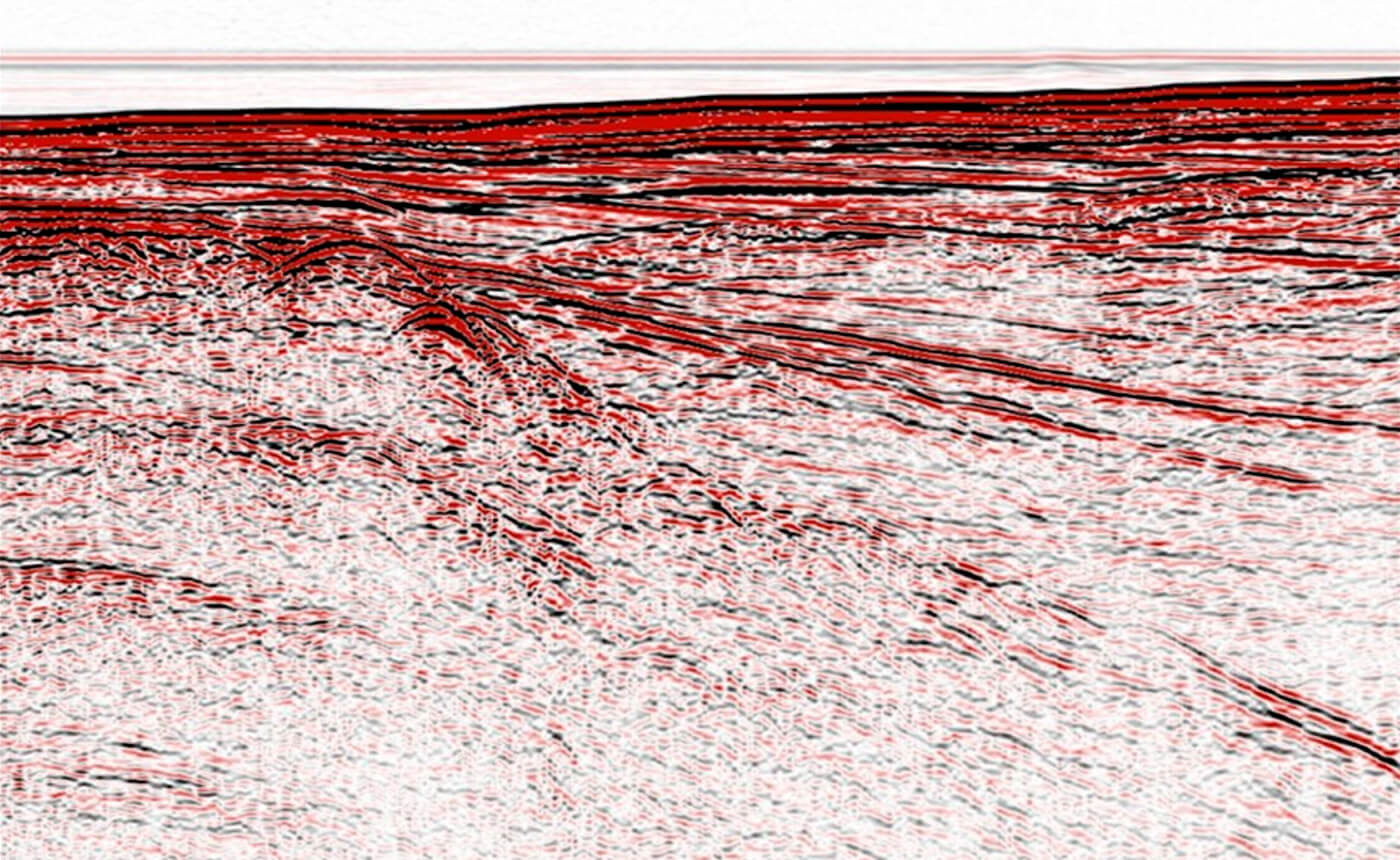
For instance, if multiples are left in a seismic section, the reflection tomographic velocity update might start chasing these lower velocities, while trying to converge to an updated velocity model solution. If the multiples are on the near offsets and are close to the main velocity trend, it might even be impossible to catch this multiple velocity trend. Proper addressing of multiples in the time processing using processes such as Surface Related Multiple Elimination (SRME) for deep water data, which utilizes modelling and adaptive subtraction of the modelled multiples, removes the multiples on the near offsets that cannot be eliminated with tau-P Radon. The better handling of noise and multiple attenuation in the time processing allows for more stable tomographic velocity updates, and faster convergence in PSDM.

We must note that recent innovations in seismic imaging allow the inclusion of multiple energy as contributing energy in the seismic processing since it can be difficult to remove multiples on the near offsets. We believe this is a very promising direction. It is still not a widely used approach, as it requires very advanced software and computational resources. If you are not planning to use the multiple energy constructively, please try to address it before taking your data into the PSDM work. The same applies to converted wave energy that is necessary in converted wave processing but has to be removed in regular P-wave processing prior to PSDM.

Preserving diffractions in pre-migration processing is critical for successful imaging results. Unfortunately, diffractions, having a non-reflection character, often get attacked and removed, even by clever and sophisticated noise attenuation algorithms such as F-XY Decon noise attenuation.

Doing due diligence in identifying your diffractions in the early processing volumes, and preserving them through your processing stages, will pay off at the depth imaging stage.

Gathering Data for Your PSDM Project: Essential, Necessary, and Sufficient

Which data should I collect for my PSDM project? We all know about the essential data, like input gathers, time processing velocities, the refraction model, etc., but what other data can benefit the PSDM project? Below, we have included a comprehensive list of data that will certainly enhance your chances of a successful PSDM outcome.

In addition to the essential seismic data, gather any other additional information you can obtain – the more the merrier.

PSDM is an integrated process that requires an integrated approach. Connect with your interpreter, geologist, petrophysicist and acquisition group. Involve your interpreters at different stages of your PSDM project and seek their input.

The following information is extremely useful for a successful PSDM project:

• A copy of the Observer’s Report (electronic format preferable)
• Acquisition maps
• Any relevant geodetic information, including any local reference frame information
• Understanding the primary objectives of the PSDM project
• Knowing the outcome and information that is expected to be gained from the PSDM data
• The target formation and its composition (geology around the target)
• Details of the overburden from the surface to the target (composition of the near-surface)
• Borehole information: logs, geologic horizon tops, descriptive reports etc.
• Structural and stratigraphic summaries of the area (with graphics)
• Petrophysical information for the area
• Well tops
• Seismic horizons
• Any previous studies of the geology in the region (previous reports)
• Are there any steep dips present in the area?
• Any known anisotropy present in the area?
• What velocity regimes are present in the section?
• Previous volumes of seismic processing
• Studies of the stress regimes and fracture networks (if such exist)
• Surface fault expressions
• Any existing information and reports on previous seismic processing in the area
• Topographic information, e.g. a Google Earth file
• Sonic and density logs
• Gamma ray log
• Caliper log
• Resistivity logs
• Check shot information, with acquisition geometry
• Deviation data, if relevant
• And last, but not least - VSP data – raw or corridor stack, if available.

The Practical Aspects of PSDM Project Execution: Are There Any Rules?

In this next section, we will go over the main aspects of PSDM project execution, and identify some useful, practical rules.

The importance of the well-defined velocity model

A PSDM can only be as good as its model (Fig. 8). This does not mean that other aspects of PSDM work are less important, but certainly, getting your velocity model right is a crucial stage of your PSDM project.

Are there any rules in velocity model building? Every experienced imager and processor will have their own tricks in their “processing hat”, but there are some commonly used practices that are a good start:

• A properly resolved near-surface is an excellent start.
• Know your initial model building options and choose your initial model building strategy, but choose wisely.
• Assess and plan for anisotropy in advance.
• Constructing an interval velocity model for PSDM requires some knowledge of the subsurface, preferably supported by well data.
• Update your model.
• Verify your model.

Addressing the near-surface is a major factor for a successful PSDM. It all starts with the shallow.

• Accurate first arrival picking is critical to the success of refraction tomographic inversion.
• An indication of the reliability of the interval velocity model from the refraction tomographic inversion can be obtained from the ray hit count. In the examples below (Figs. 9 and 10) the model is accurate to a depth of a few hundred meters.
• The velocity model from the refraction tomographic inversion may be compared to a velocity model derived from uphole surveys and other data for additional QC

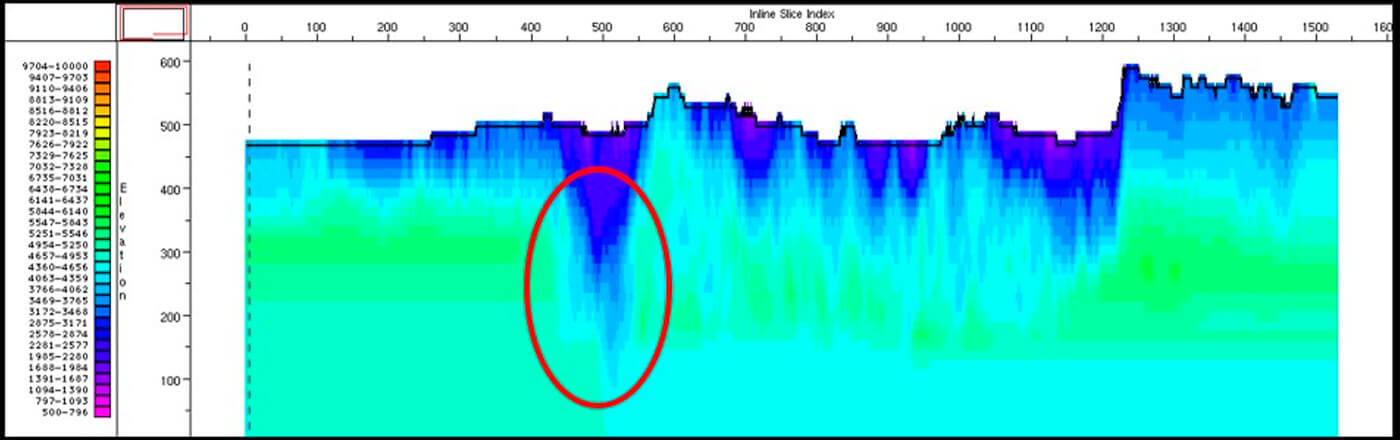
A reliable near-surface model is able to pick up shallow velocity anomalies.

A ray hit count is used for refraction model QC.

Velocity Model Building for PSDM

Initial Velocity Model

There are several ways to approach the initial Velocity Model Building (VMB). Things to avoid:

• Velocity “bullseyes”
• Sharp contrasts
• Lateral inconsistencies
• Trend that is too wild
• Trend that is too smooth.

The choice of initial velocity model directly affects the success of your PSDM project.

Let’s review three common ways of building the initial velocity model. They all have their pros and cons.

1. Wells can be used to create the interval velocity gradient and propagate it laterally. This would give a very smooth, laterally consistent model, but it can be too smooth, and too far from the actual velocity in some areas, especially if there are significant lateral velocity variations.
2. A simple compaction gradient, V = V₀ + kZ, can be used based on information provided by the interpreter or the regional trend; the benefit of this initial interval velocity is that it is very smooth, but the trend can be far from reality and will take longer to converge.
3. A smoothed time migration RMS, or NMO, velocity field is often used as a starting model. It is a very fast and easy approach to incorporate. When using this approach, the important point is that the RMS velocity should be smoothed significantly and sometimes scaled down by 10-15%. This RMS velocity field must first be converted to interval velocities, which is a potentially unstable operation akin to differentiation. Several approaches to smoothing and/or anomaly removal prior to smoothing may be required to achieve a satisfactory model. Interval velocities relate to specific geological units whereas RMS velocities don’t necessarily have any relation to the geology. If PSDM is anticipated during the PSTM process it is better that the velocities are picked with respect to seismically recognizable events, which is good practice anyway, and will result in a more stable interval velocity field. Another aspect of RMS, or NMO, velocities is that they have a horizontal component and are likely faster than the vertical interval velocities where polar anisotropy exists; hence the prior stated need to scale them down. Should any well data exist, it can be used to control the amount of scaling. Interval velocity models created in this manner should be checked for undesirable “bullseye” anomalies.

The above listed methods are not the only methods to obtain your initial velocity trend. When building your initial velocity model, you should aim to strike a balance between a proper representation of all the main velocity variations and the true geologic character of your section, while maintaining a smooth and relatively simple trend.

Velocity Model Updating

There are various methodologies for velocity model updating:

• Reflection tomographic velocity model updating and convergence
• Moveout picking on the PSDM gathers
• PSDM velocity scanning, for instance, from 80% to 120% in 2% increments. This technique is very useful when the signal-to-noise ratio on the gathers is poor. It also gives a very good idea of the sensitivity of the PSDM process to changes in the velocity field.
• Other methods.

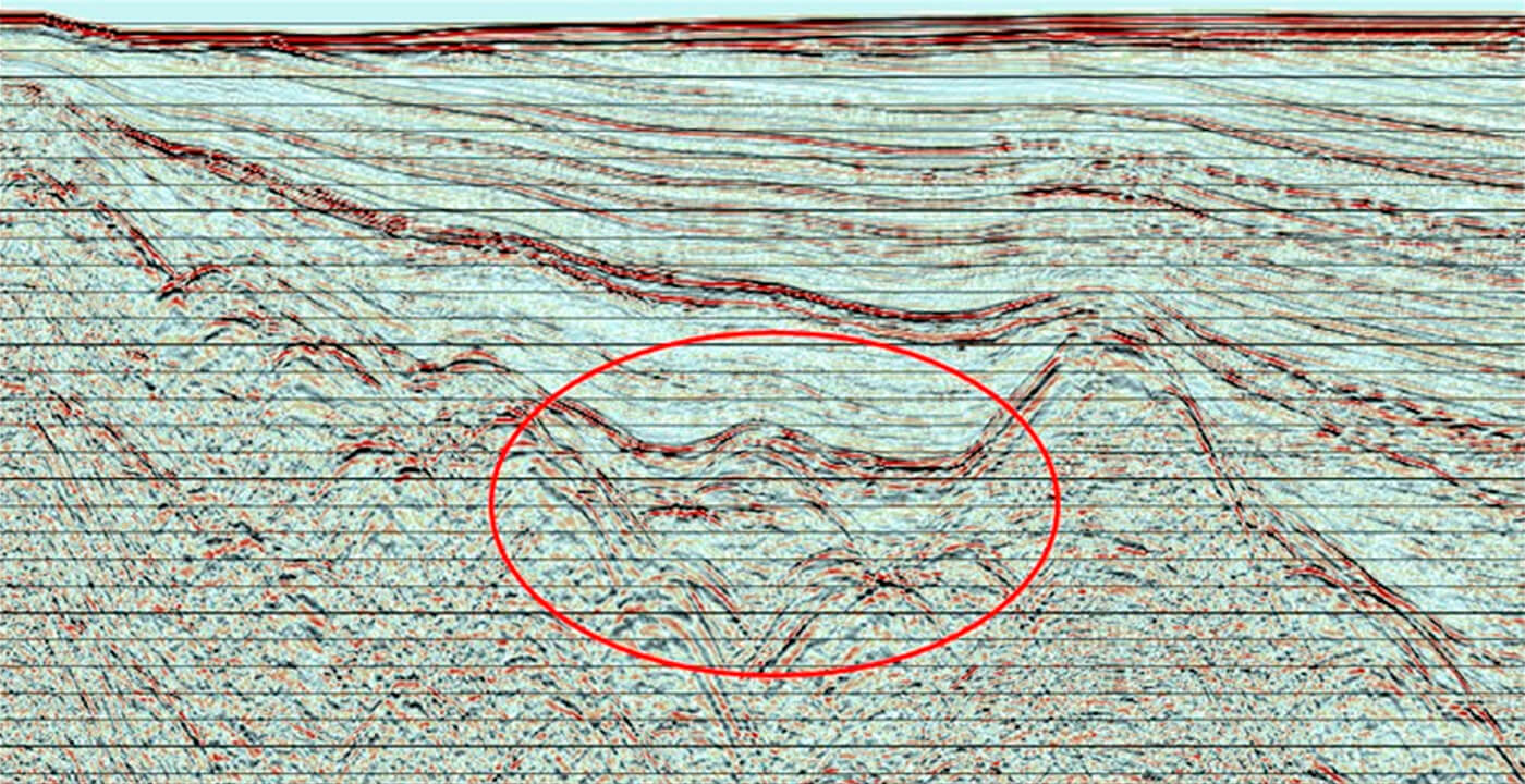
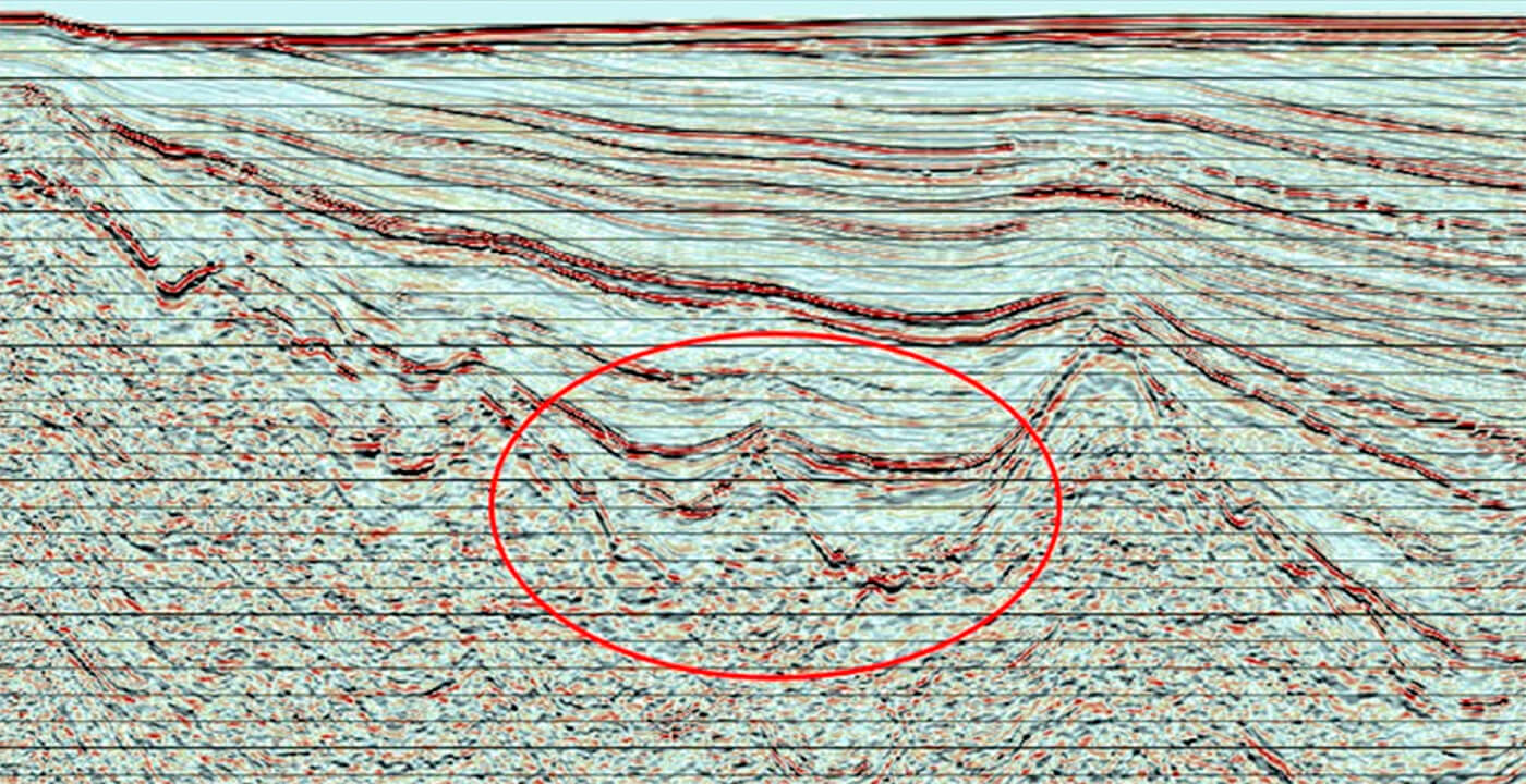
As, “It takes a village” to obtain an accurate and reliable PSDM model, these methods are often used in combination (Figs. 11 and 12). The VMB and updating is usually an iterative, comprehensive process that requires very close collaboration with interpreters and other groups.

An unreliable velocity model in PSDM defeats the whole purpose of performing PSDM.

After you have completed your thorough work on velocity updating, and migrated with the updated model, one of the main indicators of the success of your update is how well corrected are your PSDM gathers. PSDM gathers QC is one of the main QC instruments for PSDM velocity model updates. Never skip this step when QCing your PSDM updates. Selecting every n^th gather for QC allows for efficient QC of even a very large PSDM volume. The main, strongly contrasting horizons can be a good guide for efficient PSDM gathers QC.

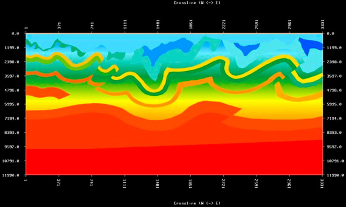
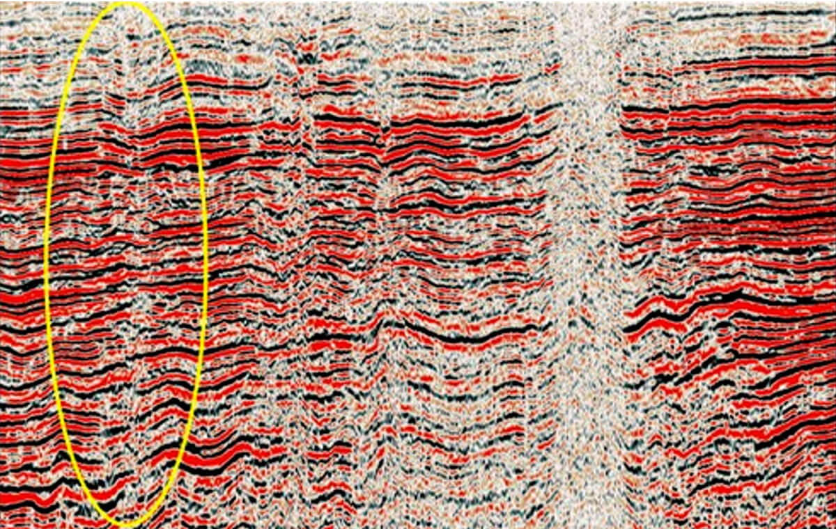
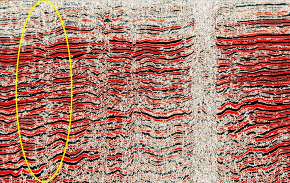
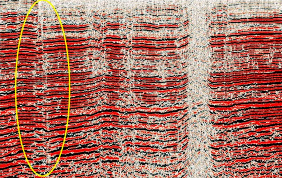
Building a velocity model in a highly structural setting

Building the velocity model in a highly structural setting is a very different “beast” (Fig. 13). It is a very tedious effort that requires iterative updates and re-migrations. The results have to be calibrated against well tops and horizons.

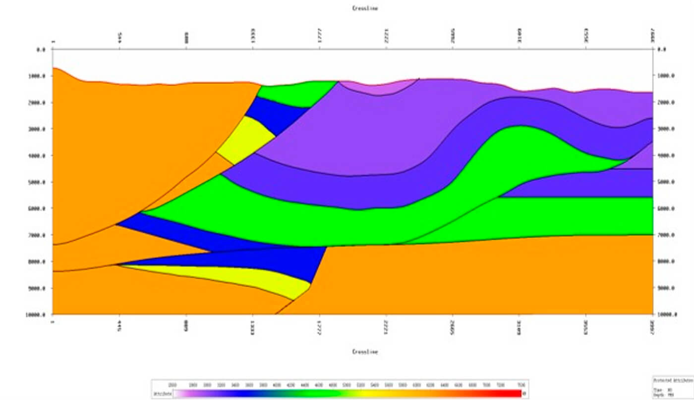
To build a velocity model in a complex setting requires much more complex and intricate work. Such velocity models are often layer-based. In addition, well tops and horizons are required to recalibrate the model at intermediate imaging stages. This work is often an iterative work project with the interpreter and integrated groups, that includes several stages of migrations, reviews, recalibrations, and adjustments followed by re-migrations. Often, it requires testing of “what if” scenarios for the uncertain layers in the model, plus additional reviews with your interpreter at various stages of the velocity model building process. This work cannot be done successfully without significant input and commitment from the interpretation group, regional knowledge, and a good understanding of the areal geology.

Anisotropy Considerations in Velocity Model Building

We will touch briefly on the subject of anisotropy, as this topic is as complex and as vast as the Universe itself. The definition below by Ian Jones gives a good idea of its complexity. We cannot not give it some attention, as it is extremely important in PSDM.

From Ian Jones:

“There are three classes of true anisotropy, some with sub-classes:

1. Intrinsic or inherent anisotropy (with 4 sub-classes):
   1. Crystalline anisotropy (with 7 crystal groups)
   2. Constraint induced (e.g. when micro-fissures are held open or closed by lithological confining pressure)
   3. Lithologically induced (e.g. Transverse Isotropy (TI) due to preferential sedimentary deposition of plate-like grains, or to plate-like crystal formation during metamorphosis)
   4. Paleomagnetically induced (during sedimentation, magnetic minerals will settle with a preferential direction. This may give rise to a detectable seismic anisotropy)
2. Crack induced anisotropy: This type of anisotropy is governed by large scale fractures which readily manifest themselves with a seismic response (this has a different form from the micro-fractures which are controlled by confining pressure)
3. Long wavelength anisotropy (with 2 sub-classes): This is a compound effect created by placing many adjacent regions together: each region itself may be isotropic, but the net effect creates a form of anisotropy. There are two sub-classes here:
   1. Periodic thin layered
   2. Checkerboard

Due to symmetries, the 81 components of the elastic compliance tensor reduce to 21; we can also have further reductions to this complexity.”

Note that in this article we are concentrating on polar anisotropy (Vertical Transverse Isotropy, VTI, and Tilted Transverse Isotropy, TTI), compressional, or P, waves and predominantly land data. Depth imaging can deal with the related Thomsen parameters, epsilon and delta, (Thomsen, 1986), plus the dip of the plane of isotropy for TTI. Time imaging works with what is known as the eta parameter introduced by Alkhalifah and Tsvankin (Alkhalifah, 1995). There is a special case termed “elliptical anisotropy” where epsilon and delta are equal and eta, with the numerator in the equation that defines it being the difference between these two parameters, will be zero and thus blind to such situations even though epsilon and delta are very likely not zero and there is indeed anisotropy. When dealing with shear waves there is a third parameter, gamma, also described in the Thomsen paper but not dealt with any further in this article.

Azimuthal anisotropy may also be a factor, especially in the presence of fractures, and is often referred to as Horizontal Transverse Isotropy or HTI. It is more than likely that VTI will coexist with HTI and this case is referred to as orthorhombic. Of course, if there is dip in the geology, quite possible when performing PSDM, then TTI and HTI may well coexist and this case is referred to as tilted orthorhombic. There is not enough space in this article to do more than make the reader aware of these forms of anisotropy (Fig. 14). There are numerous papers that discuss these higher orders of anisotropy and a good starting point for orthorhombic anisotropy would be the paper by Tariq Alkhalifah (1997), listed in References.

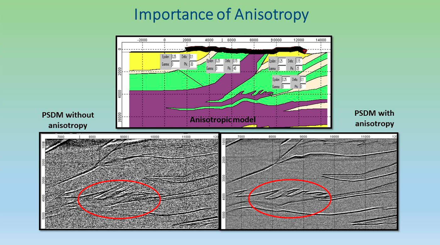
When deciding on your approach to anisotropy for your PSDM, the initial knowledge about the presence of anisotropic rocks in the section is essential. The classic anisotropic “hockey stick” is a good indication of the need for an additional polar anisotropic correction. Azimuthal anisotropy, HTI, manifests itself as sinusoidal variations with azimuth at the longer offsets, for instance in common offset common azimuth (COCA) gathers, at least in the simplest case. A velocity gradient often manifests and masquerades itself as polar anisotropy, therefore, you should always resolve your isotropic trend well, before embarking on the higher order moveout correction quest with anisotropy. A good way to do this to perform the isotropic velocity analysis first on data that has been limited to a 30 degree incidence angle; this is where offset is roughly equal to depth and the 2 term NMO approximation begins to break down.

The polar anisotropy can only be handled properly after the isotropic velocity trend is resolved in the model.

Initially obtained from petrophysics or regional knowledge, anisotropic parameters can be summarized in an anisotropy table. The parameters can then be tested through running a series of test migrations with various combinations of the proposed anisotropy pairs. Such initial anisotropy scanning provides a good starting point for your anisotropic update.

Below are some useful tips for dealing with the anisotropy on your section:

• Obtain petrophysics information.
• Use external regional information.
• Perform anisotropy scanning and confirm it with the initial migration iterations.
• Check the higher order moveout correction on the migrated sample gathers for “hockey stick” presence.
• Verify structural elements in the section (faults) – these should always be better resolved when anisotropy in the imaging is addressed properly.

Full Waveform Inversion (FWI)

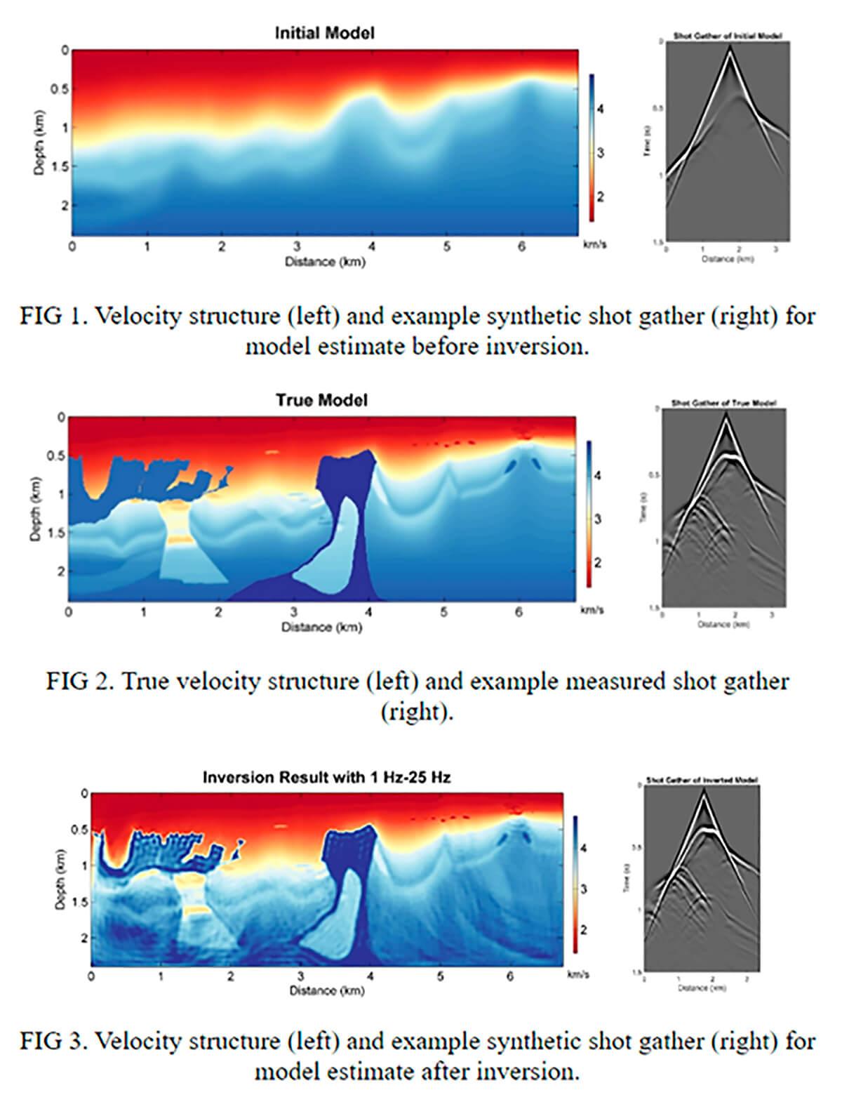
This method is still being developed and optimized for wide scale production applications. The true aim of FWI is to invert for rock properties. A few things necessary for a good velocity model from FWI are very long offsets (3X the target depth) and good low frequency signal, preferably below 2 Hz. These two criteria are not always met, especially for land data. Another often overlooked complication is density, which is often assumed to be constant or to follow Gardner's Relation, neither of which is quite right. Density is of course a factor in the reflectivity, but not in the velocity field. FWI originated with the work of Lailly (1983) and Tarantola (1984), and advances in computing technology along with the industrialization of Reverse Time Migration (RTM) have made this a feasible, though still very compute intensive, procedure. Obtaining high frequency models from FWI is very expensive, but even at 40 Hz these models are extremely accurate vertically and, perhaps more importantly, laterally, and result in images having very high definition with sharp fault indications. Velocity fields from this process may also be used in interpretive applications such as providing low frequency models for inversion or high precision velocity models for pore pressure prediction prior to drilling (Kan and Swan, 2001). Most current FWI algorithms are acoustic. Work is proceeding apace on elastic and visco-elastic versions. The reader is encouraged to follow work in these areas.

FWI is currently most often used as a velocity refinement tool and sometimes for VMB from the beginning, which can work with good quality marine data. There are many challenges with land data that are the subject of future optimizations, but we believe it has great potential to become the future tool for high resolution velocity model building (example - Fig. 15).

PSD-Migration

Setting up the grid and testing for migration parameters

For setting up your migration parameters, always rely on “tribal wisdom” but do your homework and testing. Raytracing when running a Kirchhoff-based PSDM can be modeled prior to a production run, to see how the rays behave, especially if the velocity model has sharply contrasting trends. Use your subject matter expert’s advice regarding the PSDM grid and parameters, but always test your own grid and migration parameters on a small subset of the data or selected lines before running large production volumes.

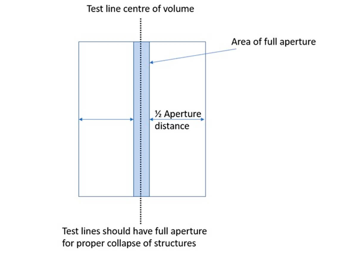
Always set and test your migration aperture and angle with your PSDM target in mind, to avoid cutting out your valuable migration energy (Fig. 16).

As the shallow part of the section often calls for detailed resolution, using variable grids (a finer, detailed grid up shallow, and a courser, more relaxed grid in the deeper part of the section), will lead to faster convergence, stabilize the migration results and enable more effective use of resources. Use your best judgement and choose the set of parameters for your final run that will allow you to optimize several things simultaneously, as in seismic inversion:

Resources + Runtime + Imaging Objectives + Resolution + Focusing

PSDM is a very resource-consuming process, and thorough pre-migration parameter testing will save re-run efforts, time and budget.

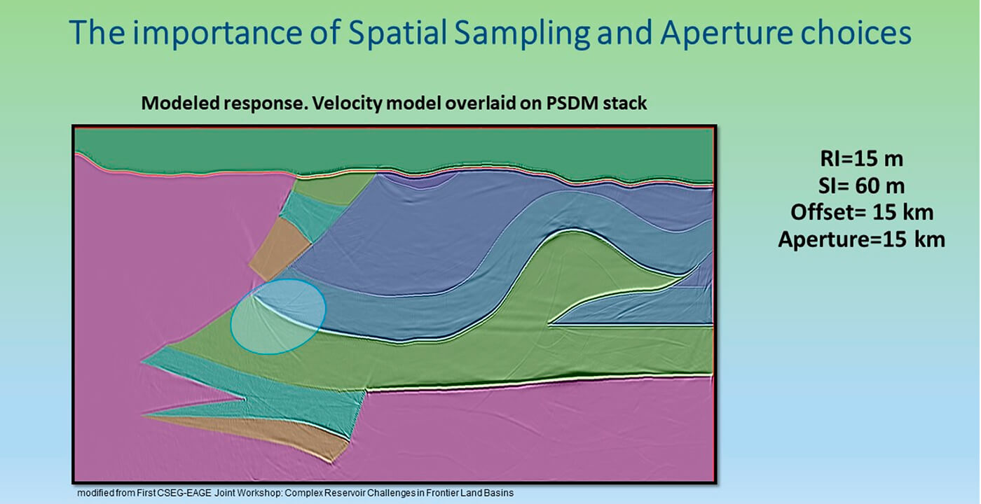
Figures 17 and 18 illustrate the importance of good spatial sampling and aperture choices. As shown in this model exercise, coarser sampling might lead to aliasing artefacts. Shorter offset and aperture may lead to insufficient imaging.

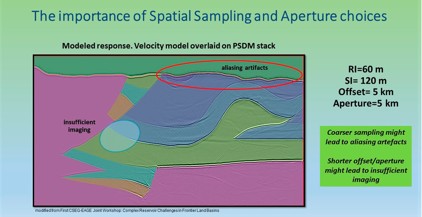
You might notice that we have gone through the better half of this article and have only now landed on migration itself. This is not because migration is not important, but because these other things are as important for a successful PSDM as migration itself and, chronologically, all of these things need to happen before you can finally migrate your volume.

If there are problems in your migration, it is possible that something went wrong way before the migration itself.

Always pick your migration method based on resource availability and imaging objectives. Good reliable Kirchhoff is often the choice at the start for onshore data, particularly structural. In onshore imaging, the more sophisticated algorithms are often utilized when you already have a good understanding of your data, through more robust migration methods.

Offshore imaging has its own preferred sequence that usually includes reverse time migration (RTM), least squares migration (LSQM), Q-migration, azimuthal imaging (for more recent wide azimuth surveys), special acquisition related methods, etc. Make sure to QC your migrated data intermittently, to avoid surprises at the end of the project.

When the volume is too large to be handled and cannot be feasibly migrated through one large run, many systems allow parallelization and simultaneous partial runs. Kirchhoff migrations may be split into common offset sub-volumes or if azimuthal anisotropy is of interest, into Common Offset Vector volumes (COV). Again, the reader is encouraged to investigate these ways of dealing with azimuthal anisotropy if they are required. The important thing is to QC the consistency of your gathered imaged data after such runs. With the modern migration algorithms, if the previously described PSDM work is done diligently, the migration itself should yield a good reliable result.

Preparing your PSDM data for future work, such as Quantitative Interpretation (QI) inversions, attributes extraction and azimuthal work, is often a requirement that you would need to carefully address, to prepare your data adequately for these next stages in the analysis process. When handing results of your PSDM work to a different group be guided by the requirements of the group or the person on the receiving end. Even the best PSDM gathers you produce might not be suitable for attribute extraction work and might require additional conditioning, noise attenuation, Radon domain treatment etc.

If the PSDM velocity model is used in the future work, it might require additional calibration with well tops and horizons and would need true vertical depth conversion. For the azimuthal work, additional migrations should be run on the data, split into desired azimuthal sectors. Common practice in the industry is to use azimuthal sectors, or alternatively COV gathers. These could potentially be split based on the regional stress regimes, or to match the acquisition in cases where the impacts of this might induce bias.

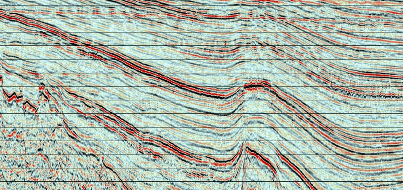
Accurate post-processing is one of the finishing touches in your imaging, and plays a vital role in your final section conditioning (Figs. 19 and 20).

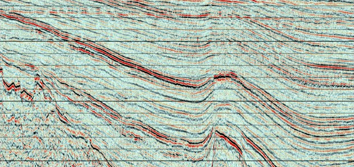
Post-processing should enhance structure but not add, create, or remove anything. When toggling between pre- and post-processed sections, it should have an affect like putting on glasses.

Showing Others What You Have Seen: Quality Control and Results Presentation

In this section we will answer the following questions:

• What are the best quality control strategies for the depth migrated volume?
• How should I manage the ever growing and multiplying output volumes?
• What about results presentation and visualization?

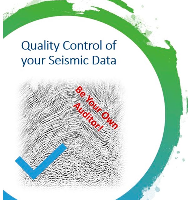
Be the auditor of your data as much as you can, and thoroughly check all the main aspects of your final PSDM output.

Once you obtain your results, the following outputs will require additional quality control:

• Near-surface imaging and resolution
• Check PSDM against the PSTM volumes
• PSDM velocity model QC
• PSDM gathers QC
• PSDM stacks QC

Imaging results plausibility are assured with:

• PSDM volumes calibration and well ties
• Main formation tops and horizon overlays
• Faults positioning and orientation

Deliverables QC include:

• Seismic and meta data QC
• SEGYs consistency and headers QC

Steps to effectively manage, anticipate, mitigate, and migrate large data volumes:

• Proactive resource allocation for anticipated large multi-trace volumes.
• Numerical verification of input and output traces at various processing stages to avoid potential trace loss.
• Comparison of the early stage migrated PSDM volumes with the final PSTM volume for structural integrity (looking for major unexplainable structural changes).
• Verification of the original inline and crossline ranges after migration.
• Interactive status updates and QC spreadsheets for managing the large production volumes (important: entries from multiple runs => one copy, single entry point).
• Generation of time slices of the full migrated volume at intermediate stages to ensure the completeness of the output data.
• Additional manual QC of seismic along inline/crossline for spatial consistency after imaging.

The art of presenting your results is as important as the work itself. Depending on which group you are presenting your results to, your presentation could be a very different presentation. It is best not to assume that your interpreters, managers, or colleagues know your material very well, even if they participated in parts of your work. If you are presenting to top management, your focus should not just be on the technical outcomes, but rather, the achieved results should be put into financial terms. Hence, turn your seismic into graphs and figures.

If only the advice from Oscar Wilde (Fig. 21) could solve all the situations with our stakeholders… Who are “they”? Anyone you present your results to: peers, group, colleagues, internal and external clients, interpreters, management, etc. It is great when feedback on your results is positive and supportive, but does it always happen? You can answer this better than anyone else.

If you performed thorough QCs at various stages of your project and verified your results, you should have good confidence and trust in your work. Several times during our careers, we were in situations when we could have agreed with the conventionally accepted version of the subsurface interpretation and not discovered more from the data. Not questioning is perhaps easier, but it does not lead to great discoveries.

Work with your interpreters and other groups to explain your results, and defend them without being defensive. Rather, understand that you all have a common goal in mind. Trust your professional instincts and help others to see what you see. And coming back to Oscar Wilde’s advice … looking at a challenging situation with some healthy humour is never a bad idea.

Time and Budget - Achieving the Unachievable

This next section is not technical, but no less significant.

One of the main problems of any PSDM project execution is often not the ambiguity of the velocity model or a wrong migration grid, but the inability of a project manager to have all the integrated parties working together in synergy.

The Project Management aspect for PSDM includes such important questions as:

• How can I estimate my budget and resources and, moreover, how can I achieve my targets?
• How many processors and imagers do I need for a given project, and how much machine time will be required?
• How can I make my resource allocation correctly?
• If something does not go as planned, what mitigation methods can we put in place, will they be enough, or will they even work?

It is important to clearly understand and define the objectives of your PSDM project at the onset and to plan and know your execution path.

The points we outline below are relevant for any project, not just PSDM. What makes a difference for a successful PSDM project executor or project manager is the ability to gather and prepare the majority of this information well before the start-up of the project, and not only that, but to communicate it effectively to all involved groups and individuals. Know your project objectives well, gather information proactively, establish your communication channels and put mitigation measures in place.

Project Initiation and Project Objectives:

• Define the overall main objectives of the exploration effort.
• Define the primary objectives of the PSDM project.
• Define any secondary objectives (if outlined) of the seismic processing project.
• Define the outcome and information that is expected to be gained from the PSDM data.
• Define the Project Plan and Scope.
• Clearly set project deadlines and resources.
• Secure IT support for the group members and software.
• Set the communication hierarchy and logistics for the communication channels.
• Assign the responsibilities of each member of the team and QC strategies.
• Plan the project risk mitigation measures if things do not go according to plan.

PSDM Project Management Tips:

• Prepare yourself by gathering all your additional information in advance.
• Know your stakeholders and establish communication channels upfront.
• Run your initial data QC, near-surface model building, and initial velocity model building in parallel to save time.
• Use selected target lines (inlines/crosslines) to optimize your migration parameters and fine tune your settings on a smaller subset before embarking on large production volume runs. Try to choose the target lines over the areas of interest or previously drilled well locations.
• Maintain an Excel spreadsheet to track the progress (testing/production).
• Good “bookkeeping” is an essential part of any PSDM project.
• Adjust the Project Scope if required for the benefit of the project, but clearly communicate the changes to all the stakeholders and receive necessary permissions and budget approval.
• QC intermediate volumes using time slices to avoid surprises at the end.
• Get your proper rest and disconnect from time to time, as large PSDM projects are extremely energy and time consuming.
• Use your subject matter experts and your interpreters as your support system.

PSDM is a complex and multi-staged process that requires an ability to adjust and adapt, as results do not always converge within the given time and budget. To focus and stay on a schedule while completing multiple complex tasks might prove to be challenging. Luckily, we, as geophysicists, embrace challenge and are well-adapted to achieving the unachievable (Fig. 22). If you follow the above-mentioned advice and tips, or design your own effective approach and strategies in advance, your PSDM project ride might be much more enjoyable.

No matter how things turn out with your project – learn, regroup, pat yourself on the back for your thorough and intelligent work and move on. You are one project older now and hence wiser and more experienced.

”Truth, like gold, is to be obtained not by its growth, but by washing away from it all that is not gold.”
- Leo Tolstoy on…geophysical processing?