Compressive sensing in seismic exploration: an outlook on a new paradigm

Part 1 of this paper is adapted from Randomized sampling and sparsity: getting more information from fewer samples. Geophysics 75, WB173 (2010); doi:10.1190/1.350614.

Abstract

Many seismic exploration techniques rely on the collection of massive data volumes that are subsequently mined for information during processing. While this approach has been extremely successful in the past, current efforts toward higher resolution images in increasingly complicated regions of the Earth continue to reveal fundamental shortcomings in our workflows. Chiefly amongst these is the so-called “curse of dimensionality” exemplified by Nyquist’s sampling criterion, which disproportionately strains current acquisition and processing systems as the size and desired resolution of our survey areas continues to increase.

We offer an alternative sampling method leveraging recent insights from compressive sensing towards seismic acquisition and processing for data that, from a traditional point of view, are considered to be undersampled. The main outcome of this approach is a new technology where acquisition and processing related costs are decoupled the stringent Nyquist sampling criterion.

At the heart of our approach lies randomized incoherent sampling that breaks subsampling-related interferences by turning them into harmless noise, which we subsequently remove by promoting sparsity in a transform-domain. Acquisition schemes designed to fit into this regime no longer grow significantly in cost with increasing resolution and dimensionality of the survey area, but instead its cost ideally only depends on transform-domain sparsity of the expected data. Our contribution is split into two part.

1 Outline

As the first portion of a two-part series, this article aims to elucidate the key principles of CS, as well as provide a discussion on how these principles can be adapted to seismic acquisition. To this end we will introduce measures that quantify reconstruction and recovery errors in order to express the overhead that CS imposes. We will then use these measures to compare the performance of different transform domains and sampling strategies during reconstruction. The second portion of this series, to appear in a later issue, will give an account of synthetic recovery experiments on a real seismic line data that utilize the ideas presented in this article, as well as consider the performance of these schemes using the measures introduced here.

1.1 Nyquist sampling and the curse of dimensionality

The livelihood of exploration seismology depends on our ability to collect, process, and image extremely large seismic data volumes. The recent push towards full-waveform approaches only exacerbates this reliance, and we, much like researchers in many other fields in science and engineering, are constantly faced with the challenge to come up with new and innovative ways to mine this overwhelming barrage of data for information. This challenge is especially daunting in exploration seismology because our data volumes sample wavefields that exhibit structure in up to five dimensions (two coordinates for the sources, two for the receivers, and one for time). When acquiring and processing this highdimensional structure, we are not only confronted with Nyquist’s sampling criterion but we also face the so-called “curse of dimensionality”, which refers to the exponential increase in volume when adding extra dimensions to our data collection.

These two challenges are amongst the largest impediments to progress in the application of more sophisticated seismic methods to oil and gas exploration. In this paper, we introduce a new methodology adapted from the field of “compressive sensing” or “compressive sampling” (CS in short throughout the article, Candès et al., 2006; Donoho, 2006a; Mallat, 2009), which is aimed at removing these impediments via dimensionality reduction techniques based on randomized subsampling. With this dimensionality reduction, we arrive at a sampling framework where the sampling rates are no longer scaling directly with the gridsize, but by transform-domain compression; more compressible data requires less sampling.

1.2 Dimensionality reduction by compressive sensing

Current nonlinear data-compression techniques are based on high-resolution linear sampling (e.g., sampling by a CCD chip in a digital camera) followed by a nonlinear encoding technique that consists of transforming the samples to some transformed domain, where the signal’s energy is encoded by a relatively small number of significant transform-domain coefficients (Mallat, 2009). Compression is accomplished by keeping only the largest transform-domain coefficients. Because this compression is lossy, there is an error after decompression. A compression ratio expresses the compressed-signal size as a fraction of the size of the original signal. The better the transform captures the energy in the sampled data, the larger the attainable compression ratio for a fixed loss.

Even though this technique underlies the digital revolution of many consumer devices, including digital cameras, music, movies, etc., it does not seem possible for exploration seismology to scale in a similar fashion because of two major hurdles. First, high-resolution data has to be collected during the linear sampling step, which is already prohibitively expensive for exploration seismology. Second, the encoding phase is nonlinear. This means that if we select a compression ratio that is too high, the decompressed signal may have an unacceptable error, in the worst case making it necessary to repeat collection of the highresolution samples.

By replacing the combination of high-resolution sampling and nonlinear compression by a single randomized subsampling technique that combines sampling and encoding in one single linear step, CS addresses many of the above shortcomings. First of all, randomized subsampling has the distinct advantage that the encoding is linear and does not require access to high-resolution data during encoding. This opens possibilities to sample incrementally and to process data in the compressed domain. Second, encoding through randomized sampling suppresses subsampling related artifacts. Coherent subsampling related artifacts, whether these are caused by periodic missing traces or by cross-talk between coherent simultaneous-sources, are turned into relatively harmless incoherent Gaussian noise by randomized subsampling (see e.g. Herrmann and Hennenfent, 2008; Hennenfent and Herrmann, 2008; Herrmann et al., 2009b, for seismic applications of this idea).

By solving a sparsity-promoting problem (Candès et al., 2006; Donoho, 2006a; Herrmann et al., 2007; Mallat, 2009), we reconstruct high-resolution data volumes from the randomized samples at the moderate cost of a minor oversampling factor compared to data volumes obtained after conventional compression (see e.g. Donoho et al., 1999 for wavelet-based compression). With sufficient sampling, this nonlinear recovery outputs a set of largest transform-domain coefficients that produces a reconstruction with a recovery error comparable with the error incurred during conventional compression. As in conventional compression this error is controllable, but in case of CS this recovery error depends on the sampling ratio, i.e., the ratio between the number of samples taken and the number of samples of the high-resolution data. Because compressively sampled data volumes are much smaller than high-resolution data volumes, we reduce the dimensionality and hence the costs of acquisition, storage, and possibly of data-driven processing.

We mainly consider recovery methods that derive from compressive sampling. Therefore our method differs from interpolation methods based on pattern recognition (Spitz, 1999), plane-wave destruction (Fomel et al., 2002) and data mapping (Bleistein et al., 2001), including parabolic, apex-shifted Radon and DMONMO/ AMO (Trad, 2003; Trad et al., 2003; Harlan et al., 1984; Hale, 1995; Canning and Gardner, 1996; Bleistein et al., 2001; Fomel, 2003; Malcolm et al., 2005). To benefit fully from this new sampling paradigm, we will translate and adapt its ideas to exploration seismology while evaluating their performance. Here lies our main contribution. Before we embark on this mission we first share some basic insights from compressive sensing in the context of a well-known problem in geophysics: recovery of time-harmonic signals, which is relevant for missingtrace interpolation.

Compressive sensing is based on three key elements: randomized sampling, sparsifying transforms, and sparsity-promotion recovery by convex optimization. By themselves, these elements are not new to geophysics. Spiky deconvolution and high-resolution transforms are all based on sparsity-promotion (Taylor et al., 1979; Oldenburg et al., 1981; Ulrych and Walker, 1982; Levy et al., 1988; Sacchi et al., 1994) and analyzed by mathematicians (Santosa and Symes, 1986; Donoho and Logan, 1992); wavelet transforms are used for seismic data compression (Donoho et al., 1999); randomized samples have been shown to benefit Fourierbased recovery from missing traces (Trad et al., 2003; Xu et al., 2005; Abma and Kabir, 2006; Zwartjes and Sacchi, 2007b). The novelty of CS lies in the combination of these concepts into a comprehensive theoretical framework that provides design principles and performance guarantees.

1.3 Examples

1.3.1 Periodic versus uniformly-random subsampling

Because Nyquist’s sampling criterion guarantees perfect reconstruction of arbitrary bandwidth-limited signals, it has been the leading design principle for seismic data acquisition and processing. This explains why acquisition crews go at length to place sources and receivers as finely and as regularly as possible. Although this approach spearheaded progress in our field, CS proves that periodic sampling at Nyquist rates may be far from optimal when the signal of interest exhibits some sort of structure, such as when the signal permits a transform-domain representation with few significant and many zero or insignificant coefficients. For this class of signals (which includes nearly all real-world signals) it suffices to sample randomly with fewer samples than that determined by Nyquist.

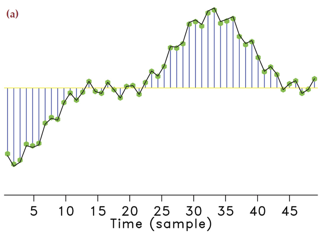
Take any arbitrary time-harmonic signal. According to compressive sensing, we can guarantee its recovery from a very small number of samples drawn at random times. In the seismic situation, this corresponds to using seismic arrays with fewer geophones selected uniformly-randomly from an underlying regular sampling grid with spacings defined by Nyquist (meaning it does not violate the Nyquist sampling theorem). By taking these samples randomly instead of periodically, the majority of artifacts directly due to incomplete sampling will behave like Gaussian white noise (Hennenfent and Herrmann, 2008; Donoho et al., 2009) message as illustrated in Figure 1. We observe that for the same number of samples the subsampling artifacts can behave very differently.

"/assets/images/articles/2011-04-compressive-sensing-fig01b.jpg"> 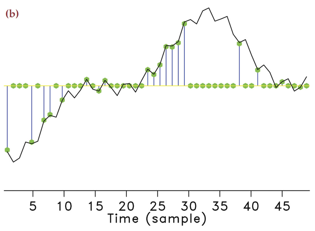"/assets/images/articles/2011-04-compressive-sensing-fig01c.jpg"> 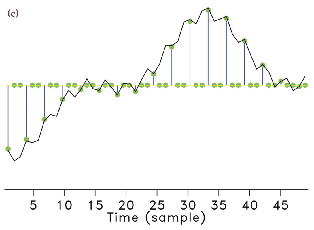"/assets/images/articles/2011-04-compressive-sensing-fig01d.jpg"> 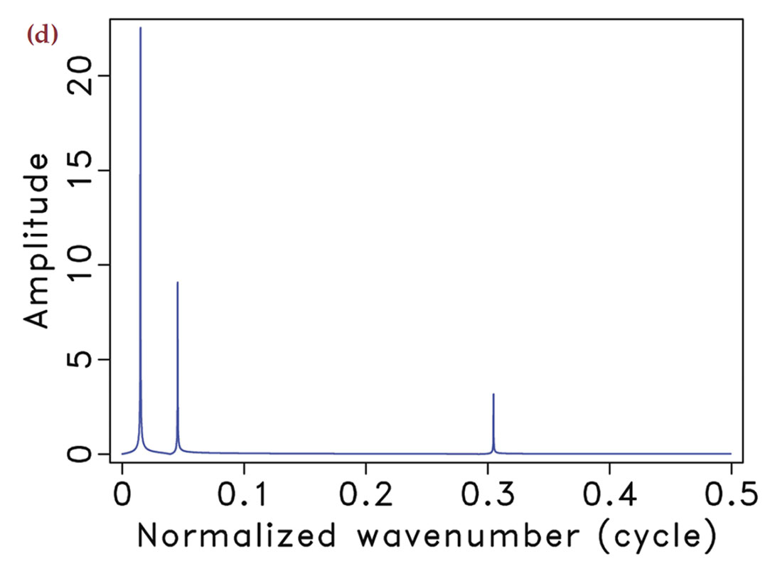"/assets/images/articles/2011-04-compressive-sensing-fig01e.jpg"> 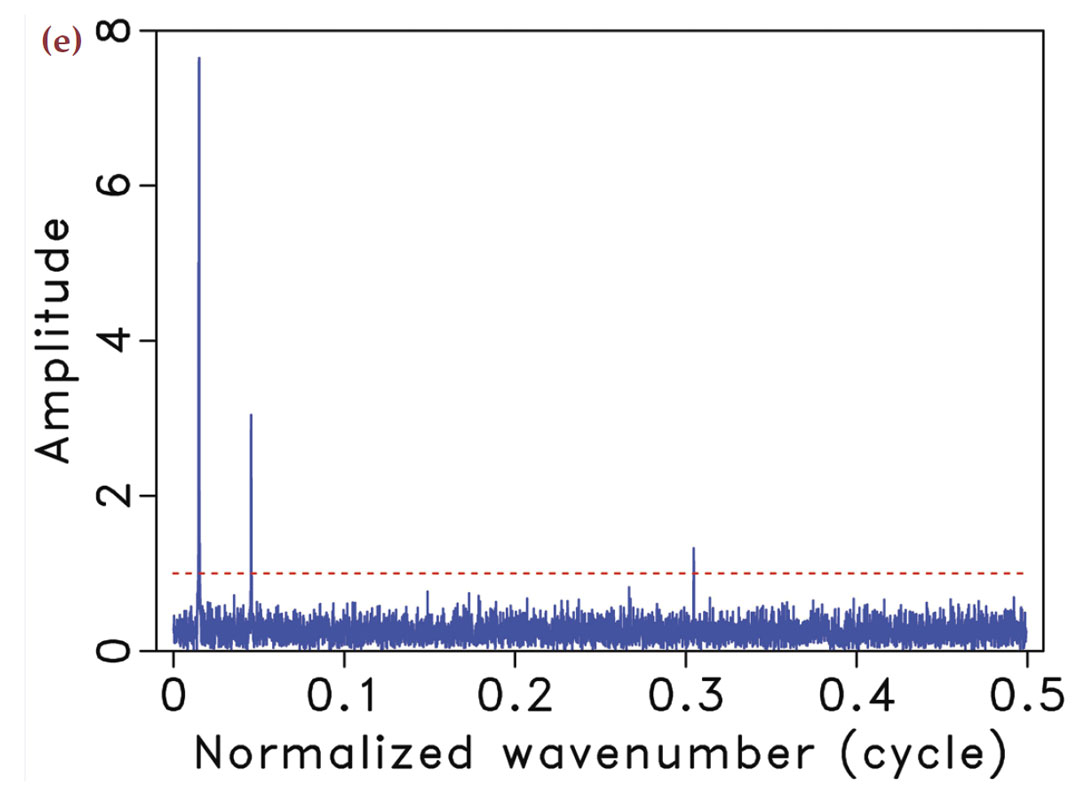"/assets/images/articles/2011-04-compressive-sensing-fig01f.jpg">

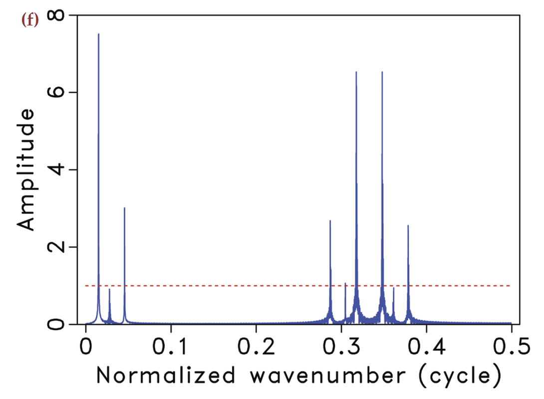
In the geophysical community, subsampling-related artifacts are commonly known as “spectral leakage” (Xu et al., 2005), where energy from each frequency is leaked to other frequencies. Understandably, the amount of spectral leakage depends on the degree of subsampling: the higher this degree the more leakage. However, the characteristics of the artifacts themselves depend on the irregularity of the sampling. The more uniformly-random our sampling is, the more the leakage behaves as zero-centered Gaussian noise spread over the entire frequency spectrum.

Compressive sensing schemes aim to design acquisition that specifically create Gaussian-noise like subsampling artifacts (Donoho et al., 2009). As opposed to coherent subsampling related artifacts (Figure 1(f)), these noise-like artifacts (Figure 1(e)) can subsequently be removed by a sparse recovery procedure, during which the artifacts are separated from the signal and amplitudes are restored. Of course, the success of this method also hinges on the degree of subsampling, which determines the noise level, and the sparsity level of the signal.

By carrying out a random ensemble of experiments, where random realizations of harmonic signals are recovered from randomized samplings with decreasing sampling ratios, we confirm this behavior empirically. Our findings are summarized in Figure 2. The estimated spectra are obtained by solving a sparsifying program with the Spectral Projected Gradient for l₁. solver (SPGL1 – Berg and Friedlander, 2008) for signals with k non-zero entries in the Fourier domain. We define these spectra by randomly selecting k entries from vectors of length 600 and populating these with values drawn from a Gaussian distribution with unit standard deviation. As we will show below, the solution of each of these problems corresponds to the inversion of a matrix whose aspect ratio (the ratio of the number of columns over the number of rows) increases as the number of samples decreases.

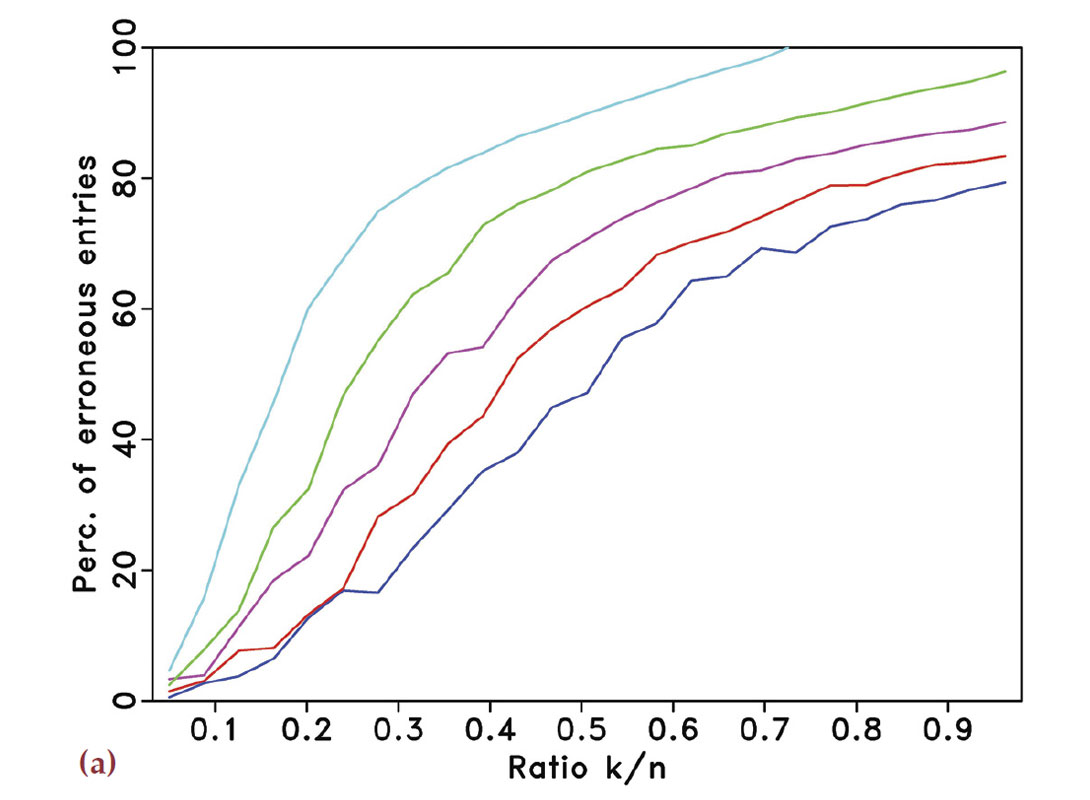
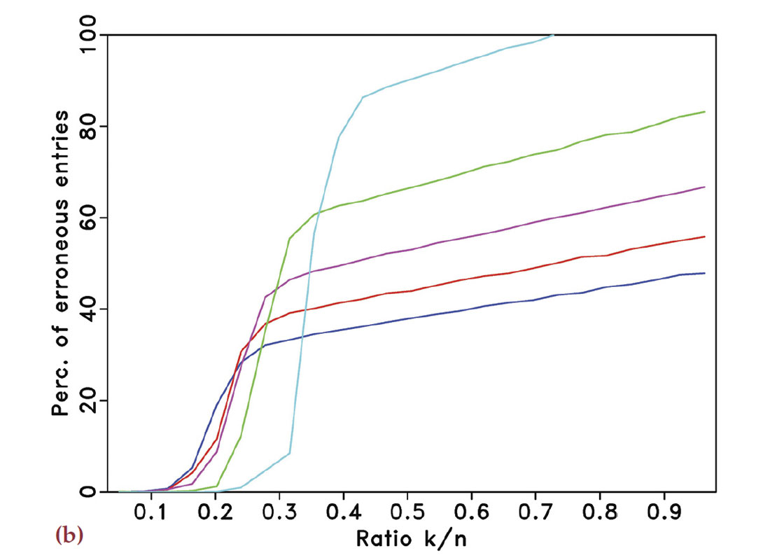
To get reasonable estimates, each experiment is repeated 100 times for the different subsampling schemes and for varying sampling ratios ranging from 1/2 to 1/6. The reconstruction error is the number of vector entries at which the estimated spectrum and the true spectrum disagree by more than 10–4. This error counts both false positives and false negatives. The averaged results for the different experiments are summarized in Figures 2(a) and 2(b), which correspond to regular and random subsampling, respectively. The horizontal axes in these plots represent the relative underdeterminedness of the system, i.e., the ratio of the number k of nonzero entries in the spectrum to the number of acquired data points n. The vertical axes denote the percentage of erroneous entries. The different curves represents the different subsampling factors. In each plot, the curves from top to bottom correspond to sampling ratios of 1/2 to 1/6.

Figure 2(a) shows that, regardless of the subsampling factor, there is no range of relative underdeterminedness for which the spectrum, and hence the signal, can accurately be recovered from regular subsamplings. Sparsity is not enough to discriminate the signal components from the spectral leakage. The situation is completely different in Figure 2(b) for the random sampling. In this case, one can observe that for a subsampling ratio of 1/2 exact recovery is possible for 0<k / n≤1/4. The main purpose of these plots is to qualitatively show the transition from successful to failed recovery. The quantitative interpretation for these diagrams of the transition is less well understood but also observed in phase diagrams in the literature (Donoho and Tanner, 2009; Donoho et al., 2009). A possible explanation for the observed behavior of the error lies in the nonlinear behavior of the solvers and on an error not measured in the l₂. sense.

1.4 Main contributions

We propose and analyze randomized sampling schemes, termed compressive seismic acquisition. Under specific conditions, these schemes create favourable recovery conditions for seismic wavefield reconstructions that impose transform-domain sparsity in Fourier or Fourier-related domains (see e.g. sacchi et al., 1998; Xu et al., 2005; Zwartjes and Sacchi, 2007a; Herrmann et al., 2007; Hennenfent and Herrmann, 2008; Tang et al., 2009). Our contribution is twofold. First, we demonstrate by means of carefully designed numerical experiments on synthetic and real data that compressive sensing can successfully be adapted to seismic acquisition, leading to a new generation of randomized acquisition and processing methodologies where high-resolution wavefields can be sampled and reconstructed with a controllable error. We introduce a number of performance measures that allow us to compare wavefield recoveries based on different sampling schemes and sparsifying transforms. Second, we show that accurate recovery can be accomplished for compressively sampled data volumes sizes that exceed the size of conventional transform-domain compressed data volumes by a small factor. Because compressive sensing combines transformation and encoding by a single linear encoding step, this technology is directly applicable to seismic acquisition and to dimensionality reduction during processing. We verify this claim by a series of experiments on real data. We also show that the linearity of CS allows us to extend this technology to seismic data processing. In either case, sampling, storage, and processing costs scale with transform-domain sparsity.

1.5 Outline

First, we briefly present the key principles of CS, followed by a discussion on how to adapt these principles to the seismic situation. For this purpose, we introduce measures that quantify reconstruction and recovery errors and expresses the overhead that CS imposes. We use these measures to compare the performance of different transform domains and sampling strategies during reconstruction. We then use this information to evaluate and apply this new sampling technology towards acquisition and processing of a 2-D seismic line.

2 Basics of compressive sensing

In this section, we give a brief overview of CS and concise recovery criteria. CS relies on specific properties of the compressive- sensing matrix and the sparsity of the to-be-recovered signal.

2.1 Recovery by sparsity-promoting inversion

Consider the following linear forward model for sampling

where b∈ ⁿ represents the compressively sampled data consisting of n measurements. Suppose that a high-resolution data f₀∈ ^N, with N the ambient dimension, has a sparse representation x₀∈ ^N in some known transform domain. For now, we assume that this representation is the identity basis - i.e., f₀ = x₀. We will also assume that the data is noise free. According to this model, measurements are defined as inner products between rows of A and high-resolution data.

The sparse recovery problem involves the reconstruction of the vector x₀∈ ^N given incomplete measurements b∈ ^N with n << N. This involves the inversion of an underdetermined system of equations defined by the matrix A∈ ^nxN, which represents the sampling operator that collects the acquired samples from the model, f₀ .

The main contribution of CS is to come up with conditions on the compressive-sampling matrix A and the sparse representation x₀ that guarantee recovery by solving a convex sparsity-promoting optimization problem. This sparsity-promoting program leverages sparsity of x₀ and hence overcomes the singular nature of A when estimating x₀ from b. After sparsity-promoting inversion, the recovered representation for the signal is given by

In this expression, the symbol ˜ represents estimated quantities and the l₁ norm ‖x‖₁ is defined as

where x[ i ] is the i^th entry of the vector x.

Minimizing the l₁ norm in equation 2 promotes sparsity in x, and the equality constraint ensures that the solution honors the acquired data. Among all possible solutions of the (severely) underdetermined system of linear equations (n << N) in equation 1, the optimization problem in equation 2 finds a sparse or, under certain conditions, the sparsest (i.e., smallest l₀ norm (Donoho and Huo, 2001) possible solution that exactly explains the data.

2.2 Recovery conditions

The basic idea behind CS (see e.g. Candès et al., 2006; Mallat, 2009) is that recovery is possible and stable as long as any subset S of k columns of the n × N matrix A with k≤ N the number of nonzeros in x, behave approximately as an orthogonal basis. In that case, we can find a constant for which we can bound the energy of the signal from above and below , i.e.,

where S runs over sets of all possible combinations of columns with the number of columns |S|≤ k (with |S| the cardinality of S). The smaller the more energy is captured and the more stable the inversion of A becomes for signals x with maximally k nonzero entries.

The key factor that bounds the restricted-isometry constants > 0 from above is the mutual coherence amongst the columns of A i.e.,

with

where a_i is the i^th column of A and ^H denotes the Hermitian transpose.

Matrices for which is small contain subsets of k columns that are incoherent. Random matrices, with Gaussian i.i.d. entries with variance n^–1. have this property, whereas deterministic constructions almost always have structure.

For these random Gaussian matrices (there are other possibilities such as Bernouilli or restricted Fourier matrices that accomplish approximately the same behavior, see e.g. Candès et al., 2006; Mallat, 2009), the mutual coherence is small. For this type of CS matrices, it can be proven that Equation 3 holds and Equation 2 recovers x₀’s exactly with high probability as long as this vector is maximally k sparse with

where C is a moderately sized constant. This result proves that for large N, recovery of k nonzeros only requires an oversampling ratio of n/k ≈ C • log₂N, as opposed to taking all N measurements.

The above result is profound because it entails an oversampling with a factor C • log₂N compared to the number of nonzeros k. Hence, the number of measurements that are required to recover these nonzeros is much smaller than the ambient dimension (n « N for large N) of high-resolution data. Similar results hold for compressible instead of strictly sparse signals while measurements can be noisy (Candès et al., 2006; Mallat, 2009). In that case, the recovery error depends on the noise level and on the transform-domain compression rate, i.e., the decay of the magnitude- sorted coefficients.

In summary, according to CS (Candès et al., 2006b; Donoho, 2006b), the solution x̃ of equation 2 and x₀ coincide when two conditions are met, namely 1) x₀ is sufficiently sparse, i.e., x₀ has few nonzero entries, and 2) the subsampling artifacts are incoherent, which is a direct consequence of measurements with a matrix whose action mimics that of a Gaussian matrix.

Unfortunately, most rigorous results from CS, except for work by (Rauhut et al., 2008), are valid for orthonormal measurement and sparsity bases only and the computation of the recovery conditions for realistically sized seismic problems remains computational prohibitive. To overcome these important shortcomings, we will in the next section introduce a number of practical and computable performance measures that allow us to design and compare different compressive-seismic acquisition strategies.

3 Compressive-sensing design

As we have seen, the machinery that supports sparse recovery from incomplete data depends on specific properties of the compressive-sensing matrix. It is important to note that CS is not meant to be blindly applied to arbitrary linear inversion problems. To the contrary, the success of a sampling scheme operating in the CS framework hinges on the design of new acquisition strategies that are both practically feasible and lead to favourable conditions for sparse recovery. Mathematically speaking, the resulting CS sampling matrix needs to both be realizable and behave as a Gaussian matrix. To this end, the following key components need to be in place:

1. a sparsifying signal representation that exploits the signal’s structure by mapping the energy into a small number of significant transform-domain coefficients. The smaller the number of significant coefficients, the better the recovery;
2. sparse recovery by transform-domain one-norm minimization that is able to handle large system sizes. The fewer the number of matrix-vector evaluations, the faster and more practically feasible the wavefield reconstruction;
3. randomized seismic acquisition that breaks coherent interferences induced by deterministic subsampling schemes. Randomization renders subsampling related artifacts, including aliases and simultaneous source crosstalk, harmless by turning these artifacts into incoherent Gaussian noise;

Given the complexity of seismic data in high dimensions and field practicalities of seismic acquisition, the mathematical formulation of CS outlined in the previous section does not readily apply to seismic exploration. Therefore, we will focus specifically on the design of source subsampling schemes that favor recovery and on the selection of the appropriate sparsifying transform. Because theoretical results are mostly lacking, we will guide ourselves by numerical experiments that are designed to measure recovery performance.

During seismic data acquisition, data volumes are collected that represent discretizations of analog finite-energy wavefields in two or more dimensions including time. We recover the discretized wavefield by inverting the compressive-sampling matrix

with the sparsity-promoting program:

This formulation differs from standard compressive sensing because we allow for a wavefield representation that is redundant, i.e., S ∈ ^PxN with P ≥ N. Aside from results reported by (Rauhut et al., 2008), which show that recovery with redundant frames is determined by the RIP constant of the restricted sampling and sparsifying matrices that is least favorable, there is no practical algorithm to compute these constants. Therefore, our hope is that the above sparsity-promoting optimization program, which finds amongst all possible transform-domain vectors the vector x̃ ∈ ^P that has the smallest l₁-norm, recovers high-resolution data f̃ ∈ ^N.

3.1 Seismic wavefield representations

One of the key ideas of CS is leveraging structure within signals to reduce sampling. Typically, structure translates into transform- domains that concentrate the signal’s energy in as few as possible significant coefficients. The size of seismic data volumes, along with the complexity of its high-dimensional and highly directional wavefront-like features, makes it difficult to find a transform that accomplishes this task.

To meet this challenge, we only consider transforms that are fast (at the most O(NlogN) with N the number of samples), multiscale (splitting the Fourier spectrum into dyadic frequency bands), and multidirectional (splitting Fourier spectrum into second dyadic angular wedges). For reference, we also include separable 2-D wavelets in our study. We define this wavelet transform as the Kronecker product (denoted by the symbol ⊗) of two 1D wavelet transforms: W = W₁ ⊗ W₁ with W₁ the 1D wavelet-transform matrix.

3.1.1 Separable versus non-separable transforms

There exists numerous signal representations that decompose a multi-dimensional signal with respect to directional and localized elements. For the appropriate representation of seismic wavefields, we limit our search to non-separable curvelets (Candès et al., 2006a) and wave atoms (Demanet and Ying, 2007). The elements of these transforms behave approximately as highfrequency asymptotic eigenfunctions of wave equations (see e.g. Smith, 1998; Candès and Demanet, 2005; Candès et al., 2006a; Herrmann et al., 2008), which makes these two representations particularly well suited for our task of representing seismic data parsimoniously.

Unlike wavelets, which compose curved wavefronts into a superposition of multiscale “fat dots” with limited directionality, curvelets and wave atoms compose wavefields as a superposition of highly anisotropic localized and multiscale waveforms, which obey a so-called parabolic scaling principle. For curvelets in the physical domain, this principle translates into a support with its length proportional to the square of the width. At the fine scales, this scaling leads to curvelets that become increasingly anisotropic, i.e., needle-like. Each dyadic frequency band is split into a number of overlapping angular wedges that double in every other dyadic scale. This partitioning results in increased directionality at the fine scales. This construction makes curvelets well adapted to data with impulsive wavefront-like features. Wave atoms, on the other hand, are anisotropic because it is their wavelength, not the physical length of the individual wave atoms, that depends quadratically on their width. By construction, wave atoms are more appropriate for data with oscillatory patterns. Because seismic data sits somewhere between these two extremes, we include both transforms in our study.

3.1.2 Approximation error

For an appropriately chosen representation magnitude-sorted transform-domain coefficients often decay rapidly—i.e., the magnitude of the j^th largest coefficient is O (j ^−S) with s≥ 1/2. For orthonormal bases, this decay rate is directly linked to the decay of the nonlinear approximation error (see e.g. Mallat, 2009). This error is expressed by

with f_k the reconstruction from the largest k – coefficients. Notice that this error does not account for discretization errors (Notice that this error does not account for discretization errors, which we ignore.)

Unfortunately, this relationship between the decay rates of the magnitude-sorted coefficients and the decay rate of the nonlinear approximation error does not hold for redundant transforms. Also, there are many coefficient sequences that explain the data f making them less sparse—i.e., expansions with respect to this type of signal representations are not unique. For instance, analysis by the curvelet transform of a single curvelet does not produce a single non-zero entry in the curvelet coefficient vector.

To address this issue, we use an alternative definition for the nonlinear approximation error, which is based on the solution of a sparsity-promoting program. With this definition, the k-term nonlinear-approximation error is computed by taking the k −largest coefficients from the vector that solves

Because this vector is obtained by inverting the synthesis operator S^H with a sparsity-promoting program, this vector is always sparser than the vector obtained by applying the analysis operator S directly.

To account for different redundancies in the transforms, we study signal-to-noise ratios (SNRs) as a function of the sparsity ratio ρ = k/P (with P = N for orthonormal bases) defined as

The smaller this ratio, the more coefficients we ignore, the sparser the transform-coefficient vector becomes, which in turn leads to a smaller SNR. In our study, we include f_ρ that are derived from either the analysis coefficients or from the synthesis coefficients. The latter coefficients are solutions of the above sparsity-promoting program (Equation 10).

3.1.3 Empirical approximation errors

The above definition gives us a metric to compare recovery SNRs of seismic data for wavelets, curvelets, and wave atoms. We make this comparison on a common-receiver gather (Figure 3) extracted from a Gulf of Suez dataset. Because the current implementations of wave atoms (Demanet and Ying, 2007) was only support data that is square, we padded the 178 traces with zeros to 1024 traces. The temporal and spatial sampling interval of the high-resolution data are 0.004s and 25m, respectively. Because this zero-padding biases the ρ, we apply a correction.

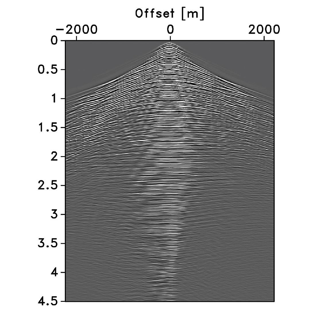
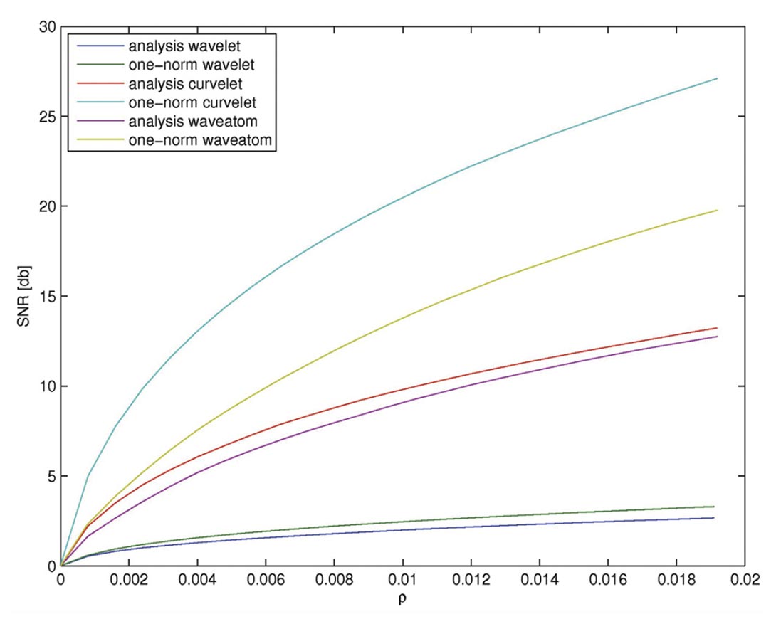
Our results are summarized in Figure 4 and they clearly show that curvelets lead to rapid improvements in SNR as the sparsity ratio increases. This effect is most pronounced for synthesis coefficients, benefiting remarkably from sparsity promotion. By comparison, wave atoms benefit not as much, and wavelet even less. This behavior is consistent with the overcompleteness of these transforms, the curvelet transform matrix has the largest redundancy (a factor of about eight in 2-D) and is therefore the tallest. Wave atoms only have a redundancy of two and wavelets are orthogonal. Since our method is based on sparse recovery, this experiment suggests that sparse recovery from subsampling would potentially benefit most from curvelets. However, this is not the only factor that determines the performance of our compressive-sampling scheme.

3.2 Subsampling of shots

Aside from obtaining good reconstructions from small compression ratios, breaking the periodicity of coherent sampling is paramount to the success of sparse recovery, whether this involves selection of subsets of sources or the design of incoherent simultaneous- source experiments. To underline the importance of maximizing incoherence in seismic acquisition, we conduct two experiments where common-source gathers are recovered from subsets of sequential and simultaneous-source experiments. To make useful comparisons, we keep for each survey the number of source experiments, and hence the size of the collected data volumes, the same.

3.2.1 Coherent versus incoherent sampling

Mathematically, sequential and simultaneous acquisition only differ in the definition of the measurement basis. For sequential-source acquisition, this sampling matrix is given by the Kronecker product of two identity bases, i.e., I := I_Ns ⊗ I_Nt, which is a N × N identity matrix with N = N_t x N_s, the product of the number of time samples N_t and the number of shots N_s. For simultaneous acquisition, where all sources fire simultaneously, this matrix is given by M := G_Ns ⊗ I_Nt with G_Ns a N_s x N_s Gaussian matrix with i.i.d. entries. In both cases, we use a restriction operator R := R_ns ⊗ I_Nt to model the collection of incomplete data by reducing the number of shots to n_s << N_s. This restriction acts on the source coordinate only.

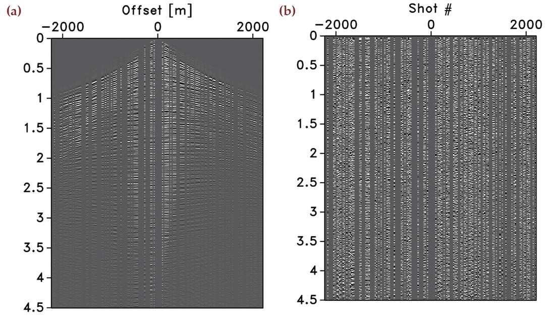
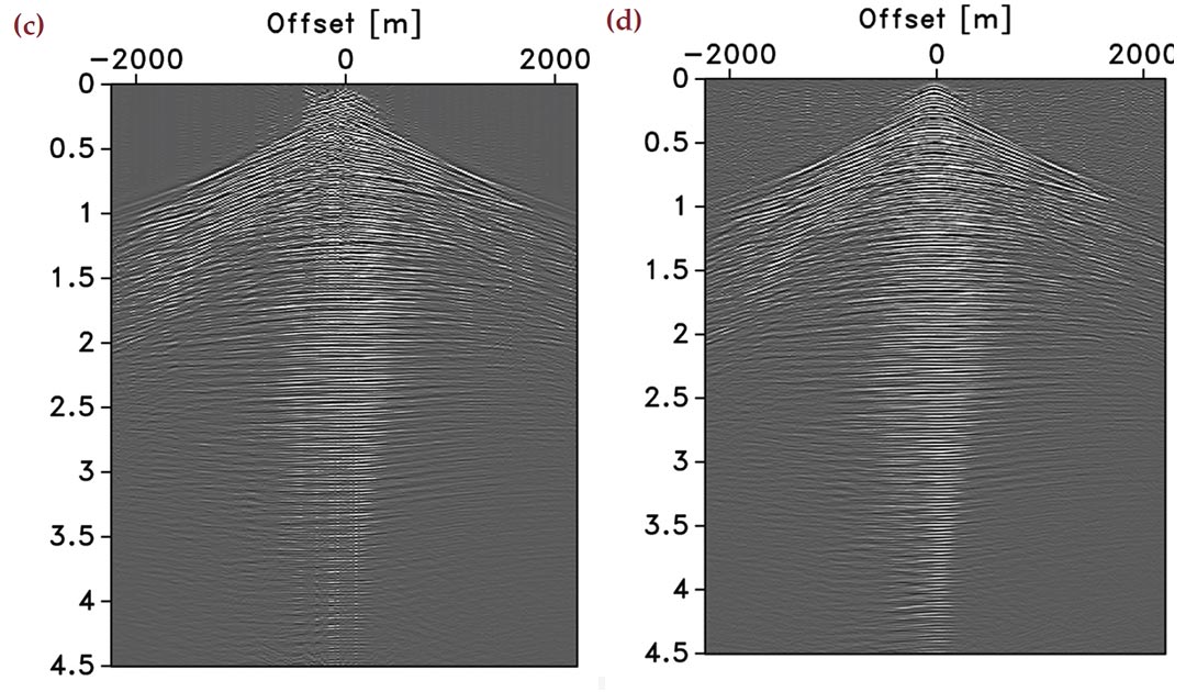
Roughly speaking, CS predicts superior recovery for compressivesampling matrices with smaller coherence. According to Equation 5, this coherence depends on the interplay between the restriction, measurement, and synthesis matrices. To make a fair comparison, we keep the restriction matrix the same and study the effect of having measurement matrices that are either given by the identity or by a random Gaussian matrix. Physically, the first CS experiment corresponds to surveys with sequential shots missing. The second CS experiment corresponds to simultaneoussource experiments with simultaneous source experiments missing. Examples of both measurements for the real common-receiver gather of Figure 3 are plotted in Figure 5(a) and 5(b), respectively. Both data sets have 50% of the original size. Remember that the horizontal axes in the simultaneous experiment no longer has a physical meaning. Notice also that there is no observable coherent crosstalk amongst the simultaneous sources.

Multiplication of orthonormal sparsifying bases by random measurement matrices turns into random matrices with a small mutual coherence amongst the columns. This property also holds (but only approximately) for redundant signal representations with synthesis matrices that are wide and have columns that are linearly dependent. This suggests improved performance using random incoherent measurement matrices. To verify this statement empirically, we compare sparse recoveries with Equation 8 from data plotted in Figures 5(a) and 5(b).

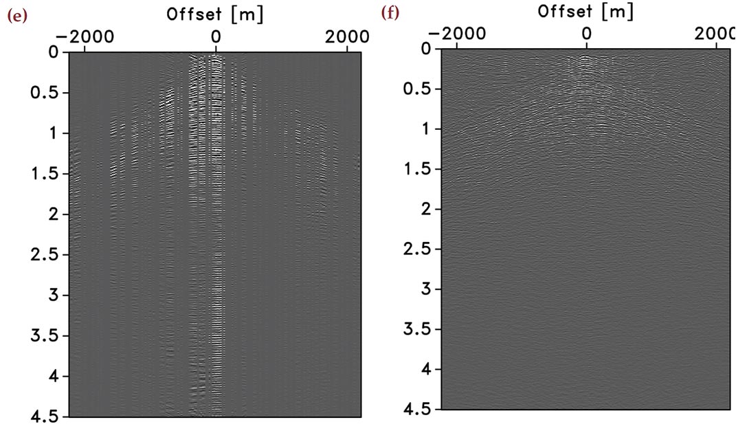
Despite the fact that simultaneous acquisition with all sources firing simultaneously may not be easily implementable in practice (although one can easily imagine a procedure in the field where a “supershot” is created by some stacking procedure), this approach has been applied successfully to reduce simulation and imaging costs (Herrmann et al., 2009b; Herrmann, 2009; Lin and Herrmann, 2009a, b). In the “eyeball norm”, the recovery from the simultaneous data is as expected clearly superior (cf. Figures 5(c) and 5(d)). The difference plots (cf. Figures 5(e) and 5(f)) confirm this observation and show very little coherent signal loss for the recovery from simultaneous data. This is consistent with CS, which predicts improved performance for sampling schemes that are more incoherent. Because this qualitative statement depends on the interplay between the sampling and the sparsifying transform, we conduct an extensive series of experiments to get a better idea on the performance of these two different sampling schemes for different sparsifying transforms. We postpone our analysis of the quantitative behavior of the recovery SNRs to after that discussion.

3.2.2 Sparse recovery errors

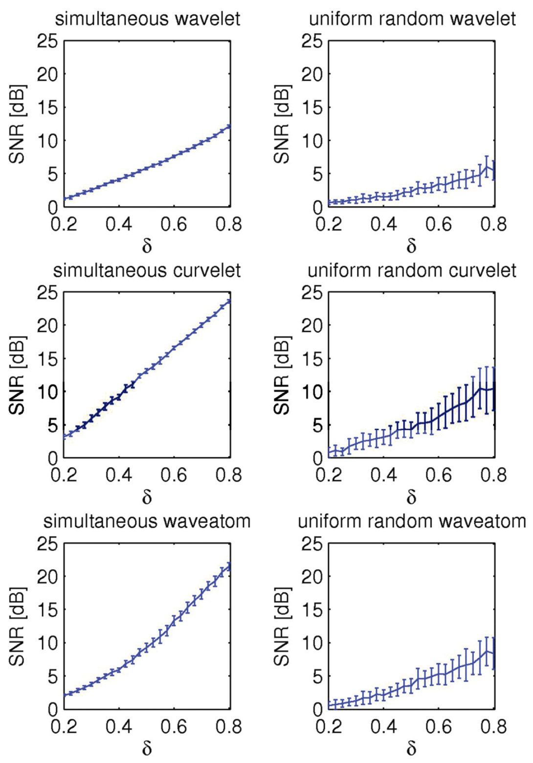
The examples of the previous section clearly illustrate that randomized sampling is important, and that randomized simultaneous acquisition leads to better recovery compared to randomized subsampling of sequential sources. To establish this observation more rigorously, we calculate estimates for the recovery error as a function of the sampling ratio δ = n/N by conducting a series of 25 controlled recovery experiments. For each δ ∈ [0.2, 0.8], we generate 25 realizations of the randomized compressive-sampling matrix. Applying these matrices to our common-receiver gather (Figure 3) produces 25 different data sets that are subsequently used as input to sparse recovery with wavelets, curvelets, and wave atoms. For each realization, we calculate the SNR(δ) with

For each experiment, the recovery of f̃ _δ is calculated by solving this optimization problem for 25 different realizations of A_δ with A_δ := R_δM_δS^H, where R_δ := R_ns ⊗ I_Nt with δ = n_s/N_s. For each simultaneous experiment, we also generate different realizations of the measurement matrix M := G_Ns ⊗ I_Nt .

From these randomly selected experiments, we calculate the average SNRs for the recovery error, SNR(δ), including its standard deviation. By selecting δ evenly on the interval δ ∈ [0.2, 0.8], we obtain reasonable reliable estimates with error bars. Results of this exercise are summarized in Figure 6. From these plots it becomes immediately clear that simultaneous acquisition greatly improves recovery for all three transforms. Not only are the SNRs better, but the spread in SNRs amongst the different reconstructions is also much less, which is important for quality assurance. The plots validate CS, which predicts improved recovery for increased sampling ratios. Although somewhat less pronounced as for the approximation SNRs in Figure 4, our results again show superior performance for curvelets compared to wave atoms and wavelets. This observation is consistent with our earlier empirical findings.

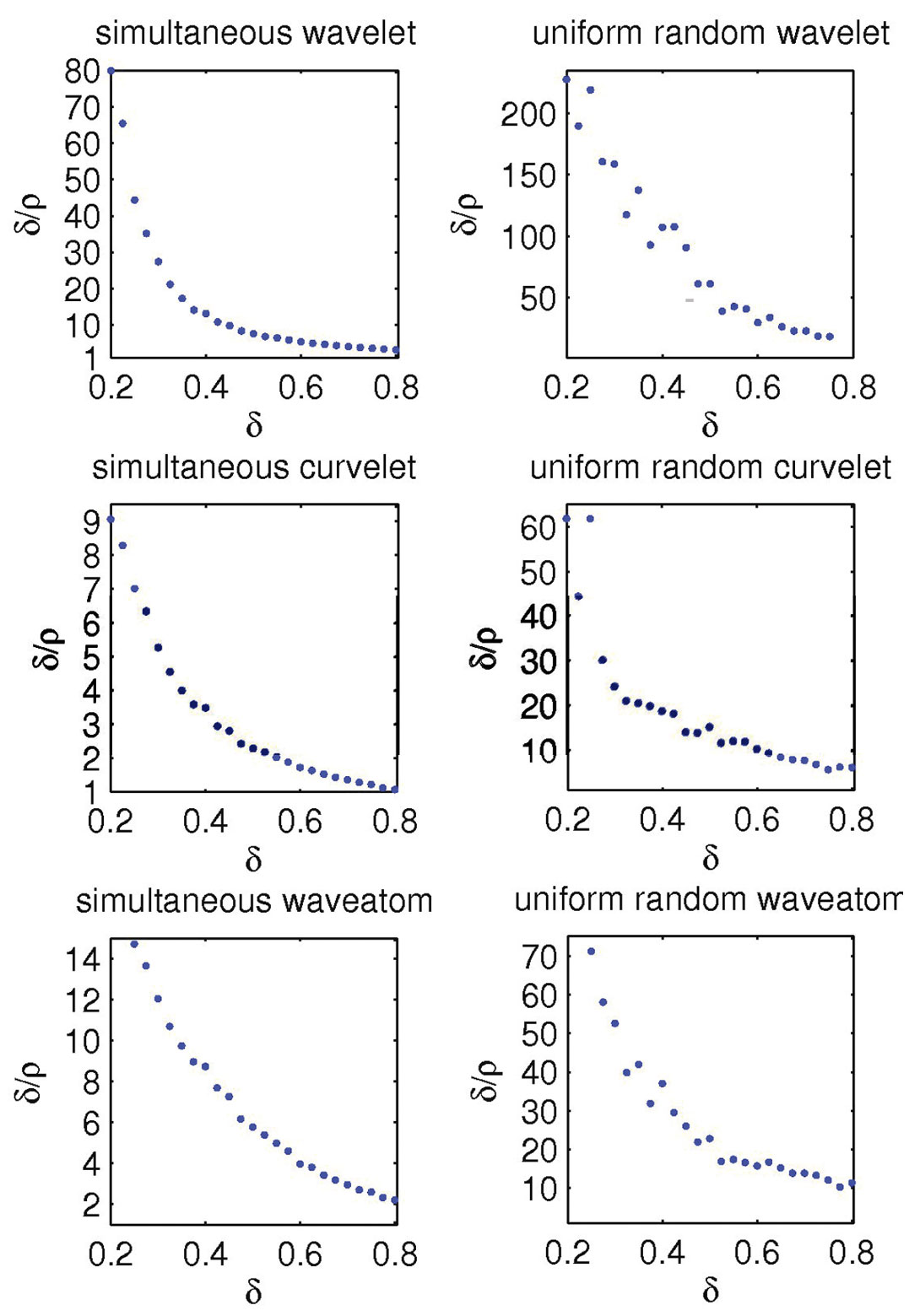
3.2.3 Empirical oversampling ratios

The key factor that establishes CS is the sparsity ratio ρ that is required to recover wavefields with errors that do not exceed a predetermined nonlinear approximation error (cf. Equation 11). The latter sets the fraction of largest coefficients that needs to be recovered to meet a preset minimal SNR for reconstruction.

Motivated by (Mallat 2009), we introduce the oversampling ratio δ/ρ ≥ 1. For a given δ, we obtain a target SNR from SNR(δ). Then, we find the smallest ρ for which the nonlinear recovery SNR is greater or equal to SNR(δ). Thus, the oversampling ratio δ/ρ ≥ 1 expresses the sampling overhead required by compressive sensing. This measure helps us to determine the performance of our CS scheme numerically. The smaller this ratio, the smaller the overhead and the more economically favorable this technology becomes compared to conventional sampling schemes.

We calculate for each δ ∈ [0.2, 0.8]

When the sampling ratio approaches one from below (δ → 1), the data becomes more and more sampled leading to smaller and smaller recovery errors. To match this decreasing error, the sparsity ratio ρ → 1 and consequently we can expect this oversampling ratio to go to one, δ/ρ → 1.

Remember that in the CS paradigm, acquisition costs grow with the permissible recovery SNR that determines the sparsity ratio. Conversely, the costs of conventional sampling grow with the size of the sampling grid irrespective of the transformdomain compressibility of the wavefield, which in higher dimensions proves to be a major difficulty.

The numerical results of our experiments are summarized in Figure 7. Our calculations use empirical SNRs for both the approximation errors of the synthesis coefficients as a function of ρ and the recovery errors as a function of δ. The estimated curves lead to the following observations. First, as the sampling ratio increases the oversampling ratio decreases, which can be understood because the recovery becomes easier and more accurate. Second, recoveries from simultaneous data have significantly less overhead and curvelets outperform wave atoms, which in turn perform significantly better than wavelets. All curves converge to the lower limit (depicted by the dashed line) as δ →1. Because of the large errorbars in the recovery SNRs (cf. Figure 6), the results for the recovery from missing sequential sources are less clear. However, general trends predicted by CS are also observable for this type of acquisition, but the performance is significantly worse than for recovery with simultaneous sources. Finally, the observed oversampling ratios are reasonable for both curvelet and wave atoms.

4 Conclusions

Following ideas from compressive sensing, we made the case that seismic wavefields can be reconstructed with a controllable error from randomized subsamplings. By means of carefully designed numerical experiments on synthetic and real data, we established that compressive sensing can indeed successfully be adapted to seismic data acquisition, leading to a new generation of randomized acquisition and processing methodologies.

With carefully designed experiments and the introduction of performance measures for nonlinear approximation and recovery errors, we established that curvelets perform best in recovery, closely followed by wave atoms, and with wavelets coming in as a distant third, which is consistent with the directional nature of seismic wavefronts. This finding is remarkable for the following reasons: (i) it underlines the importance of sparsity promotion, which offsets the “costs” of redundancy and (ii) it shows that the relative sparsity ratio effectively determines the recovery performance rather than the absolute number of significant coefficients. Our observation of significantly improved recovery for simultaneous-source acquisition also confirms predictions of compressive sensing. Finally, our analysis showed that accurate recoveries are possible from compressively sampled data volumes that exceed the size of conventionally compressed data volumes by only a small factor. In part II, we will adapt these findings to a seismic line by comparing the recovery performance in case of ‘Land’, via randomly-weighted simultaneous sources, and ‘Marine’ acquisition, via individual sources going off at random times and at random locations.

Acknowledgements

This paper was written as a follow up to the first author’s presentation during the “Recent advances and Road Ahead” session at the 79th. annual meeting of the Society of Exploration Geophysicists. I would like to thank the organizers of this session Dave Wilkinson and Masoud Nikravesh for their invitation. I also would like to thank Dries Gisolf and Eric Verschuur of the Delft University of Technology for their hospitality during my sabbatical and Gilles Hennenfent for preparing some of the figures. This publication was prepared using CurveLab, a toolbox implementing the Fast Discrete Curvelet Transform, WaveAtom a toolbox implementing the Wave Atom transform, Madagascar, a package for reproducible computational experiments, SPGl₁, SPOT, a suite of linear operators and problems for testing algorithms for sparse signal reconstruction, and pSPOT, SLIM’s parallel extension of SPOT. FJH was in part financially supported by NSERC Discovery Grant (22R81254) and by CRD Grant. The industrial sponsors of the Seismic Laboratory for Imaging and Modelling, BG Group, BP, Chevron, ConocoPhillips, Petrobras, Total SA, WesternGeco are also gratefully acknowledged.