An efficient 3D explicit finite-difference prestack depth migration

Summary

An explicit, constrained operator is presented here for wavefield extrapolation in 3D wave equation depth migration. The migration cost and image quality benefit from its reduced number of independent coefficients within the operator, negligible numerical anisotropy, and flexibility that allows for different propagation angles and step sizes in the inline and cross-line directions. In order to further reduce the computational workload we dynamically select operator lengths and extrapolation step sizes based on the wavenumber of the wave components being migrated. The phase-shifted linear interpolation that we propose for interpolating the extrapolated wavefield is suitable for the explicit migration, and significantly improves the accuracy of the result when compared with the linear interpolation typically used in implicit migrations.

Introduction

Downward extrapolation of the seismic wavefield is the key element of wave equation based migrations because it determines the image quality and computational cost. Extrapolation by finite difference methods is considered to be superior, especially in handling lateral velocity variations. It can be classified into explicit and implicit methods. Accomplished simply by convolving known wavefields with an extrapolation operator, the explicit method is easier to implement, and can be more efficient than the implicit method. In addition, the explicit method can be extended to 3D in a straightforward manner, whereas the implicit method requires inline and crossline splitting of the extrapolation process at each depth step, resulting in phase errors and artifacts.

Even with symmetrical operators (Blacquiere et al., 1989), 3D depth migrations based on explicit extrapolation may still be expensive, due to a full 2D convolution being performed at each depth. The scheme based on the McClellan transform proposed by Hale (1991) is much more efficient, but introduces numerical anisotropy at the same time. Among the many alternatives, or improvements to the scheme (Soubaras, 1992; Sollid and Arntsen, 1994; Biondi and Palacharla, 1995; Mittet, 2002), the constrained operator proposed by Mittet (2002) is attractive. It overcomes the numerical anisotropy problem and still keeps the computational cost comparable to the Hale-McClellan scheme.

Method and Results

Constrained operator

As demonstrated in Figure 1, the explicit finite-difference operator is separated into two areas during the operator design. The operator is a function of the local wavenumber at each output grid location, and is able to handle lateral velocity variations. As usual for explicit finite-difference migration operators, the operator assumes a circular symmetry. What is unique about the operator presented here is that it divides the coefficients into core and constrained areas. In the core area the coefficient layout is the same as that for a full operator. In the constrained area the coefficients in a series of rings are assigned an identical value. Figure 1 shows the layout of a constrained operator with the Δy/Δx ratio of 1.5, x-direction half-length of 12, y-direction half-length of 8, and core half-length of 6.

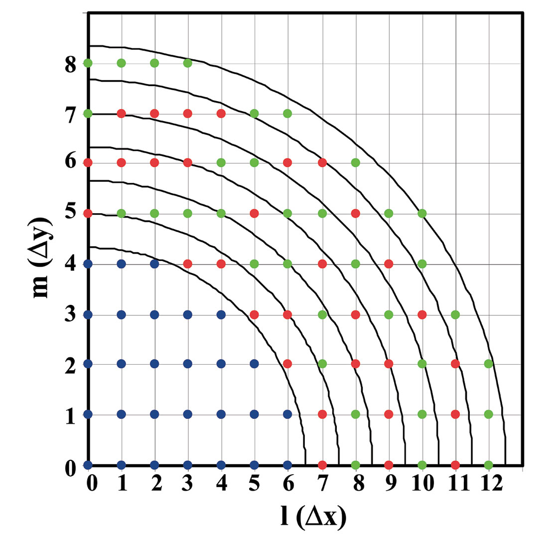
The constrained operator reduces the number of independent coefficients. By factorizing out the coefficients in a ring during the convolution, the number of complex multiplications is reduced. Because the complex multiplication is expensive, using the constrained operator improves the extrapolation efficiency.

The operator half-length, M, in the y direction, is determined from the operator half-length, L, in the x direction, using the relationship M=(Δy/Δx)L. If Δy is greater than Δx, as is usually the case for marine acquisition, the total number of operator coefficients and the computational cost is reduced.

The coefficients of the constrained operator are designed using the exact extrapolator in the frequency-wavenumber domain, that is, the phase shift operator. The design strategy is to optimize the constrained operator such that its wavenumber-domain response approaches that of the exact phase shift operator. For any given local wavenumber, the optimization is performed on the operator’s real and imaginary parts, using an L8 norm for all inline and cross-line wavenumbers (k_x and k_y) up to the critical wavenumber

determined by:

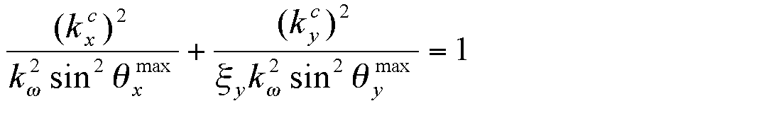
where are the maximum propagation angles considered in the x and y directions.

are the maximum propagation angles considered in the x and y directions.

We design the constrained operator for a sufficient set of kw and form an operator table. For a given accuracy, the operator length required varies with kw. Our extrapolation process selects the shortest operator that satisfies the accuracy required based on the wavenumber value of the wave component being migrated. This measure avoids using unnecessarily long operators, and can reduce computational cost.

Variable extrapolation step size and interpolation

To reduce the number of extrapolations we use a variable step size that is determined dynamically by the wavenumber value. To interpolate the extrapolated wavefield onto a regular output depth grid we propose a phase-shifted linear interpolation. We do not consider the linear interpolation used in implicit migrations where the interpolation is performed only on the “diffraction” term, and the “thin-lens” term is calculated exactly. In an explicit migration those two terms are not separated, and the use of linear interpolation on the “thin-lens” term will generate a large error. The phase shifts are applied to each extrapolated wavefield frequency prior to the linear interpolation to the output depth grid, and eliminate the influence of the “thin-lens” term.

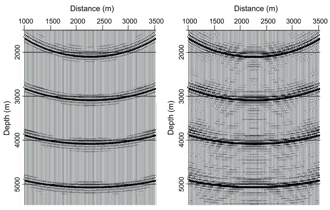
Figure 2 shows a part of the source wavefield snapshot obtained with the constrained operator and phase-shifted linear interpolation. The extrapolation interval is 25 m and the interpolation interval is 5 m. The source function used contains 4 wavelets with a flat frequency spectrum between 1 – 39 Hz. The model has a constant velocity of 2000 m/s. The wavefield obtained with the phase-shifted linear interpolation is clean, and does not have obvious amplitude distortions and phase errors. For comparison, also shown in Figure 2, is the result obtained with linear interpolation. We note that the linear interpolation generates strong noise cutting through the wavefronts, and obvious amplitude distortions and phase errors can be observed, especially around the low dip portions of the wavefront.

Examples

To illustrate the performance of the explicit 3D wave equation migration, we have applied it to the SEG/EAGE salt model dataset. Figure 3 compares Kirchhoff and explicit finite-difference migrations. In comparison to Kirchhoff migration, the image from the wave equation migration has a lower noise level, does a better job imaging the salt boundaries, and, most importantly, it produces a much more focused and continuous image.

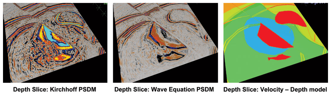
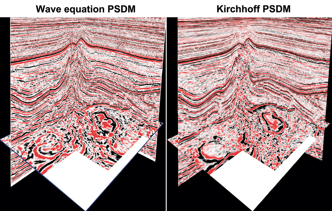
We have also applied the explicit wave equation migration to a real dataset from the southern North Sea (Figure 4). Not only does the explicit finite-difference migration yield significantly better steep dip imaging in the centre area of the example shown, but the coherency and resolution of low dip events are also much better than the Kirchhoff result. A thin, high-velocity chalk layer confronts imaging quality for deeper events in this region, as evidenced in the Kirchhoff result.

Conclusions

The constrained operator is accurate and reliable for wavefield extrapolation in explicit depth migrations. The smaller number of independent coefficients offered by the operator leads to a reduced migration computational cost. Its flexibility to allow for a larger grid interval and shorter operator length in the cross-line direction makes it a useful and efficient method for migrating marine data. The measures we take, including the dynamic selection of the operator length and extrapolation step size based on the wavenumber, also contribute to the efficiency of the method. The phase-shifted linear interpolation method proposed for interpolating the extrapolated wavefield is suitable for explicit migration, and is more accurate than the linear interpolation.

Acknowledgements

The authors would like to thank Rune Mittet and John Anderson for their useful suggestions and discussions. We also thank Sandy Carroll, Boris Tsimelzon and Peter Wijnen for their assistance with processing.

This article is based on the Best Petroleum Paper which was presented by Andrew Long at the 17th ASEG Conference and Exhibition, held in Sydney during August 2004. It was first published in the October 2004 issue of the ASEG's Preview magazine and is re-published here with permission of the ASEG.