A Gentle Introduction to Machine Learning

Machine learning has generated a lot of excitement in recent years. It is only a matter of time before machine learning becomes commonplace in geoscience. There are many reasons for this that I could argue, but two come immediately to mind:

• machine learning has enjoyed incredible success in similar data-rich domains, and
• you are already using it.

In spite of this, machine learning remains a slightly uncomfortable and obscure topic for some in the geoscience community. A rift has developed between geoscience and data science, in part, due to different curricula during training for each field and also some stark differences between the cultures of industries each field is hired into. A dizzying lexicon describing some very complicated mathematics and algorithms have not helped. However, I expect that each of you is far more familiar with machine learning than you suppose. Many of you are probably aware that you interface with machine learning each time you use a search engine, use word suggestion while text messaging, or shop online. You may be aware that machine learning is now being used in data security, fraud detection, computer vision, healthcare, financial trading, gaming, marketing, natural language processing, and for many other applications. You are likely engaging with machine learning products many times every day.

Of course, a passive interaction with machine learning doesn’t really count. Everyone does that. What may surprise you most, however, is that, as a geophysicist, you have probably been using machine learning throughout your career. Did you know that linear regression is machine learning? Spatial interpolation is machine learning? Seismic inversion is machine learning?

What IS machine learning?

The key word in machine learning is, of course, ‘learning’. If human learning is knowledge acquired through experience, study, or being taught, how does a machine learn? Tom Mitchell proposed this formal definition of machine learning:

What does this mean?

When given a method to make predictions based on structures that represent information in data, a program is able to learn something about the data [2]. Learning, then, is a slightly disingenuous way to describe the process of machine learning; generalization is more accurate. In the words of Adam Gibson and Josh Patterson,

The purpose of machine learning is to make predictions. If we can test the predictions of a generalization, or model, and can make changes to improve (or worsen) performance, then we can build a better predictive algorithm. For example, a Sweet Spot identified at a vertical well location is associated with a set of seismic attributes (features) at that location. If the attributes used to solve for the Sweet Spot locally are available globally, Sweet Spot locations can be predicted throughout the remainder of the seismic data. If a Sweet Spot characterized at a single well location is provided to a machine learning algorithm, the predictive power of the resulting model may be poor. If 20 new wells are drilled at locations selected by the model, many of the predictions might be wrong. However, if the model is refreshed with data from the 20 new wells, an improved model can be created.

On the other hand, a process that performs a task because its programmer has predefined the relationship between a function and its data does not learn. The performance of such a process will not change no matter how many times it executes a task, how a user engages it, or what data it is provided. For example, a process that identifies brittle rock via a predetermined relationship – an empirical formula or scalar transform – between lambda-rho and mu-rho is not machine learning. The outcome for each data point is not affected by the remainder of the data, only the predetermined relationship. I’m not suggesting that such a program is not good, only that it is not machine learning.

So then, how do you test whether or not a machine is learning? First, perform the process in question on a small data set. The results will serve as a benchmark. To test whether a program learns, simply remove a subset of the data – even a single data point – and run the process again; if the output of the process matches the benchmark run exactly, the program has not learned. If the results are different, even if only slightly, it has learned. Significantly, if it has learned, the accuracy of its output can be improved with more data and better training techniques.

Machine learning is rooted in probability theory and statistics. Machine learning only uses the data it has been provided to make predictions. The importance of this idea cannot be overstated; it has never been easier to demonstrate the value of data, great or little, to managers and decision-makers than it is with machine learning techniques.

Problem-solving with machine learning

A large variety of approaches to machine learning have been developed to address an equally wide variety of problems. Understanding which machine learning approach is effective for your problem is essential to success and tantamount to doing the work itself. Machine learning methods can be subdivided in a number of ways: algorithm architecture, loss function, learning style, label data type, and so on. However, for readers new to machine learning, it is simplest to categorize machine learning by the data set you have (inputs) and by the kind of data you want to end with (outputs). Figure 1 illustrates machine learning categorized by the kinds of problems commonly solved by geophysicists.

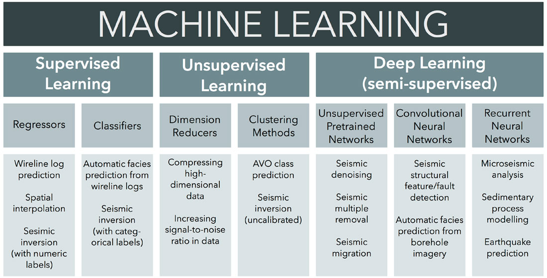
Learning style is best explained by characterizing its end members: supervised and unsupervised learning. Supervised learning is the most popular and best-understood learning style. Supervised learning uses data with labels and performance is measured by a model’s ability to predict labels accurately. The outputs of supervised learning are numerical labels (e.g., Young’s Modulus) or categorical labels (e.g., AVO class). Unsupervised learning uses data without labels and, therefore, performance must be measured differently. Like supervised learning, the outputs of supervised learning are numerical or categorical values, but, because they are absent from the inputs, explicit labels cannot be predicted. An unsupervised method, clustering, is frequently featured in rock physics and seismic reservoir characterization problems to predict groupings based on structures within data. A third learning style, mainly associated with deep learning, is often referred to as semi-supervised. Semi-supervised learning uses data with labels to produce a model, but limits user interaction with some processes operating in hidden layers, where features are commonly selected and manipulated by unsupervised methods.

Machine learning fundamentals

Since machine learning finds answers directly from data via mathematical operations, an understanding of machine learning begins with understanding data in mathematical terms.

Scalars. A scalar is the most basic element in a set of data, given as a value to represent a specific position – a sample – in that field. A scalar is a quantity: a real number. An example of a scalar is a sample measured at a depth z from a density log.

Vectors. A vector is an ordered set of n scalars. In machine learning, a vector represents a point in n-dimensional space, which can be visualized as a Euclidean distance from the origin to the point represented by the vector. For example, several samples measured at depth z: density, p-, and s-sonic, form a 1 x 3 vector, a one-dimensional array.

Matrices. A matrix is an ordered set of n vectors of equal dimension. For example, density, p-, and s-sonic values measured at several depths, z1, z2, z3, z4, form a 3 x 4 matrix, a two-dimensional array.

Tensors. Scalars, vectors, and matrices are special cases of arrays (of rank 0, 1, and 2, respectively). A more general case of an array with n-dimensions (rank n) is called a tensor. Problems appropriate for shallow learning (i.e. not deep learning) methods commonly have two-dimensional data and, therefore, are represented by a matrix. More complex data such as imagery, represented by 3 or more dimensions (x-position, y-position, and one or more attributes associated with an xy-position), are called tensors.

Linear algebra. N-dimensional tensors are common to all machine learning problems. Linear algebraic operations: the dot product, the element-wise (Hadamard) product, and outer product, are used to solve machine learning problems.

Each of these objects and operations is fundamental to nearly every aspect of machine learning, from the simplest algorithm to the most complex. Equipped with these ideas, we will explore the main families of algorithms used to solve common geophysical problems of different types (Figure 1).

Supervised learning

Solving for labels with features. In supervised learning, labels refer to values that are estimated by models. Features are values used to build a model which will predict labels. This is a very common family of problem in geophysics and includes spatial interpolation, wireline log-to-log prediction, and seismic inversion for continuous properties. For example, Bruno Ruas de Pinho solves a spatial interpolation problem with several supervised learning methods in a tutorial-style blog post [3]. To understand how this is done, consider a problem of the form:

Ax = b

where A and b are n-dimensional tensors and x is a coefficient. The constituents of A are features and those of b are labels. In supervised learning, A is usually a matrix (i.e. two-dimensional with n-variables) and b and x are vectors (i.e. one-dimensional). Implicitly, A and b are known, so we solve for x. If we can create a system of equations where x is a single coefficient, the equation takes the form:

A^-1b = x

where A^-1 is the inverted tensor A. Note that this equation represents the solution itself, not a method for its calculation. A wide variety of algorithms – processes or sets of rules followed in problem-solving operations – can be used to create a model and a model is responsible for predicting labels.

Features and labels can be numerical or categorical. Some algorithms, such as decision trees, are very versatile and can be used to solve problems with numerical features and labels, categorical features and numerical labels, numerical features and categorical labels, categorical features and labels, or some combination of numerical and categorical features and numerical or categorical labels. Many algorithms are not so versatile; however, most regression algorithms can be modified with logistic regression to solve problems with categorical labels.

Regression. A regression function attempts to predict real (numerical) values of the dependent variable (i.e. the label) from one or more independent variables (i.e. features) in a data set. The most basic form of regression is linear regression, which takes the form:

Ax = b – c

where A is a matrix of independent variables (features), b is a vector (labels), x is a parameter vector, and c is a constant that satisfies the equation when Ax = 0.

Feature engineering and selection. The equation Ax = b – c forms a straight line, which you might think is not particularly useful. However, linear regression can often be used on nonlinear data after the raw data are transformed. For example, a logarithmic, exponential, or polar coordinate transformation of a feature will generate a new feature that forms a linear relationship with a label. The process of calculating new features from raw data to create a set of more useful features is called feature engineering. Feature selection, which refers to any number of processes that select a subset of features from matrix A, is commonly used together with feature engineering to improve the results of a model.

Optimizing a model. We have described linear regression algebraically; however, we have not considered how to optimize the fit of a linear regression model to the data. A well-fit model will predict label values that match the true labels very closely. To solve for a line of best fit in a linear regression problem, we use the familiar equation:

ŷ = ax_i + b

where ŷ = ax_i + b where ŷ is a line with slope a and intercept b, which is brought as close as possible to each y_i for i = 1, 2, … , N

We can get very close to optimization by simply 'eyeballing' a best fit line through a number of points. However, in machine learning, we must calculate a solution using a cost function. The most basic cost function is the sum of squared errors:

Written in terms of a and b, we have:

To minimize E, we take partial derivatives with respect to a and b and set them to zero. This gives us a system of two equations, which can then be used to solve for a and b. Note that in this case, a and b are the parameter vector x.

Training set. A supervised learning model is calculated directly from features and labels of a data set. These are referred to as the training set.

Testing set. A testing set is not used to create the model and instead used to measure the performance of a model. A true testing set is data not-yet-acquired; however, in practice, a testing set is a subset of available data.

Overfitting and underfitting. It is possible to find a model so well-fit that every data point in the training set is predicted accurately, but it is unlikely that such a model will be useful for estimating purposes. A good model will accurately predict labels for the previously unseen features of a testing set. Such a model is said to have a low generalization error (out-of-sample error). However, many models are overfit or underfit. A model is overfit when it becomes sensitive to noise or bias in the training sample. As a result, an overfit model will accurately predict labels from the training data but will not accurately predict labels from a testing set. On the other hand, an underfit model will neglect too much of the complexity present in a training set, resulting in a high generalization error.

Regularization. Regularization is a process of tuning a model to a preferred level of complexity in order to solve an ill-posed problem or to prevent overfitting. Regularization algorithms are commonly modified regression models, which apply penalties to reduce the influence of outliers or complexities of a model.

Classification. As mentioned above, labels in supervised learning problems can be numerical or categorical. Classification is used to predict a categorical label value (e.g., lithology prediction from wireline logs [4]). A classification model, at its simplest, produces a binary output with labels of two classes: 0 and 1. Some models, e.g., decision trees, create a binary output directly. Other models calculate a probability (value between 0 and 1) and separate the values according to a threshold value, commonly 0.5 with a discriminant function. Multiclass or multinomial classification is usually achieved with a one-versus-one or one-versus-all process. The prior fits one discriminant per class pair, whereas the latter fits a discriminant for each class of the output.

Logistic regression. Logistic regression, in spite of its misleading name, is a linear function used for classification. The function has a shape of a sigmoid, asymptotically approaching both 0 and 1. The output of the logistic regression function is a probability. A linear discriminant function is fit to the data to minimize loss (error). Logistic regression is a very popular classifier: it can produce a binary or probability output and can be bolted onto a variety of regression algorithms to produce a binary output.

Decision boundaries. As in logistic regression, methods that use a decision boundary are driven by a linear function. However, the output of a decision boundary method is one of two classes rather than a probability [5]. Two classes in n-dimensional space are divided by an (n-1)-dimensional feature called a hyperplane. A popular method called the support vector machine (SVM) uses a decision boundary. The basic function of the SVM is to separate support vectors, or points in n-dimensional space, of different classes by a hyperplane with a margin of maximal width.

Cross-validation. In practice, optimal models are impossible because a true testing set is never a priori knowledge. For this reason, it is very important to use a training set as effectively as possible. The process of cross-validation, where a subset of the training set is withheld and treated as a testing set, is used to assess how a model will perform in practice. A randomly selected population from the training set may be biased, i.e. it may characterize the full training set poorly; for this reason, it matters how the training set is partitioned for cross-validation. Any of a number of partition strategies can be employed in cross-validation: random split, leave-P-out, stratified shuffle split, to name a few. To reduce variability, multiple rounds, or k-folds, of cross-validation are usually performed using different partitions.

Measuring performance. True performance is never really known. Performance measures are, in fact, estimates. The more complete a data set is and the higher the quality its acquisition, the closer a performance measure comes to the truth. Regression loss metrics are borrowed directly from statistics: variance, mean absolute error, mean squared error, mean squared logarithmic error, median absolute error, r2 (coefficient of determination), etc. Classification metrics are, at once, simpler and more complicated: simpler in their calculations and more complicated in divining their meaning. The result of a classification, illustrated by a confusion matrix, is one of four outcomes; a true positive, a false positive, a true negative, and a false negative. These are the four outcomes of conditional probability, as formalized in Bayes’ Theorem (for a nice visualization of this, visit http://setosa.io/ev/conditional-probability/) [6]. Accuracy is the ratio of correct predictions to all predictions. This metric, while important, does not tell the whole story. The aptly-named precision metric refers to the ratio of true positives to true and false positives and evaluates a classifier’s precision. The recall metric is the ratio of true positives to false negatives, which evaluates the classifier’s completeness. The F1 score, calculated

2 (precision * recall) (precision + recall)^-1

measures a balance between precision and recall, which is often a very effective metric to evaluate a classifier’s performance [7].

Unsupervised learning

Unsupervised learning seeks to exploit natural structures in unlabeled data. It is not obvious that they would be, but unsupervised methods are extremely useful for geophysicists, especially subsurface interpreters. Unsupervised learning will present an interpreter with considerable opportunity for authorship and will be increasingly used as a supplement to interpretation methods. For example, Lassock and Sansal’s work on prestack sparse azimuthal AVO inversion, where attributes extracted using the azimuthal inversion are clustered using an unsupervised learning algorithm [8]. There are two families of problems commonly solved with unsupervised learning methods: dimensionality reduction and clustering.

Dimensionality reduction. Dimensionality reduction algorithms reduce the number of features under consideration by describing the same data with fewer features along unsupervised dimensions of high variance. The purpose of performing dimensionality reduction on data is to increase data efficiency: to save on computational expense and to strengthen the signal-to-noise ratio by eliminating dimensions high in noise or low in variance in data. The outputs of dimensionality reduction can be used as inputs for another generalizing regression or classification algorithm.

A frequently unwanted consequence of the unsupervised nature of these algorithms is the destruction of the original features. For example, if you have meticulously calculated a number of rock properties from seismic data and are interested in knowing which ones are the best at detecting a mechanical rock facies, an unsupervised dimensionality reducer is not the right tool for you (you would be better served by any number of feature selection tools). Some of the more popular dimensionality reduction methods are:

• Principal component analysis (PCA)
• Singular value decomposition (SVD)
• Linear discriminant analysis (LDA)
• Quadratic discriminant analysis (QDA)
• Factor analysis (FA)
• Independent component analysis (ICA)

Many of these methods have multiple variants and can be adapted for use in classification and regression problems. For a very effective visual explanation of principal component analysis, go to http://setosa.io/ev/principal-component-analysis/ [9].

Clustering. Clustering of unlabeled data is a process of organizing vectors into classes populated by members who are similar in some way. K-centroids are iteratively moved toward a position in n-dimensional feature space, where a density function for vectors is maximized. After the process is complete, vectors are grouped with the class of the nearest centroid. The method of distance calculation varies between algorithms and produces significantly different results. Consequently, different algorithms are appropriate for different use cases, which are described in terms of the distribution and geometry of vectors in n-dimensional feature space. Some of the more commonly used clustering methods are:

• K-means
• Fuzzy c-means
• Spectral
• Ward
• Gaussian mixtures
• Birch

For a fantastic interactive tool for visualizing K-means clustering, go to https://www.naftaliharris.com/blog/visualizing-k-means-clustering/ [10].

While unsupervised learning methods use data with no labels, the outputs are still predictions and there are a number methods for performance evaluation. For dimensionality reduction methods, metrics are centred on variance. For clustering methods, most metrics focus on one of two concepts: similarity within clusters and difference between clusters.

Deep learning

Deep learning is responsible for much the recent advances in machine learning. It is noteworthy that deep learning is particularly effective at solving problems involving data that can be described as high-dimensional tensors. A significant proportion of geoscience problems involve just that sort of data: 3-D seismic data, rock imagery, and microseismic data, to name a few. Deep learning will impact the future of geoscience.

Neural networks. Deep learning methods evolved from the neural network, which is inspired by the structure and function of biological neurons. The neural network has been around since the 1960s and has developed in fits and starts.

As with linear regression, an equation of the form Ax = b can be used to describe a neural network. Here, A still represents a matrix of features and b remains a vector of labels. However, instead of a coefficient, weights on the neural network connections become the parameter vector x. The behaviour of a neural network is dependent on its architecture: the number of neurons, number of layers, and the connections between layers. Even very simple neural network architecture can represent any function if provided with enough neurons, layers, and connections [11].

Backpropagation. Neural networks are trained using the backward propagation of errors, or backpropagation. Beginning at the output and working backwards through hidden layers, backpropagation uses gradient descent (the derivative of a loss function) with respect to the neural network’s weights of the neural connections x to minimize error.

Deep learning. Deep learning is commonly based directly on simpler neural network architecture and driven by of a handful of linear regression functions. However, increases in neurons and layers, more complex ways of connecting those neurons and layers, and exponentially greater computing power have resulted in a class of very powerful learning models [12]. Deep learning often exploits unsupervised learning methods in hidden layers to drive efficiency or automatic feature extraction. These hybrid learning styles are referred to as semi-supervised learning.

For good results, deep learning methods require training with a lot of data. Additionally, and similarly to neural networks, deep learning methods are profoundly influenced by network architecture. As a result, solutions to different kinds of problems emerge from different network architectures. We will briefly examine three: unsupervised pretrained networks, convolutional neural networks, and recurrent neural networks.

Unsupervised pretrained networks (UPNs). Generally-speaking, UPNs are very good at reproducing input data or generating outputs that share a likeness with inputs. UPNs can be further subdivided into three distinct architectures:

• Autoencoders
• Deep Belief Networks (DBNs)
• Generative Adversarial Networks (GANs)

Autoencoders are used as powerful dimensionality-reducers. The output of the autoencoder network is a reconstruction of the input in its most efficient form. Autoencoders differ from many other neural networks based on multilayer perceptron architecture in that:

• they perform unsupervised learning with unlabeled data and
• they construct a compressed representation of the input [12].

DBNs consist of layers of Restricted Boltzmann Machines (RBMs). The RBM is a generative stochastic artificial neural network that can learn a probability distribution over its set of inputs [13]. An RBM can approximate an input using a series of stepped sigmoid units, or binary layers of equal weight but progressively stronger negative bias [14]. The RBM has been improved by rectified linear units (ReLU), which share the same architecture but preserve information about relative intensities through successive layers [14]. Layering RBMs allows a DBN to progressively learn more complex features automatically and, with adequately deep layering, generate convincing reproductions of inputs.

GANs. A GAN is a system of two neural networks competing in a zero-sum game and consists of:

• a generative model that estimates data distribution of a training set and
• a discriminative model that estimates the probability that a sample came from the training set rather than the generative model [15].

A GAN is able to keep a parameter count significantly smaller than other methods with respect to the amount of data used to train the network. After being trained, GANs have performed well when called upon to synthesize related, but novel, images. Graham Ganssle’s work, in this issue, on image-to-image translation with a deep convolutional GAN demonstrates how this technique can be used for seismic denoising [16].

Convolutional neural networks (CNNs). CNNs are a powerful method for computer vision. The CNN uses convolution, a mathematical operation describing a rule for merging two sets of information, to learn features in data automatically. A CNN consists of a number of hidden layers where convolution filters of various size and configurations are passed across the width, height, and depth of an input volume in strides, in the fashion of a sliding window. The architecture of a CNN is one of restricted connectivity [17] characterized by one or more convolutional layers alternately-stacked with spatial pooling layers, which serve to compress data in the network. A CNN is organized so that learned filters produce the strongest activation to spatially local input patterns. The result of this: filters are learned that will activate on features only when they occur in their respective field of reception [18]. With greater network depth, filters can recognize increasingly complex features and do so globally [13].

Similar to other neural networks, weights in a CNN are optimized with a backpropagation technique. However, as overfitting can frustrate the performance of a CNN, backpropagation is calculated on networks generated by one or more regularization methods. Of the most effective of these, called dropout, thins the network by dropping neurons (and their connections) during training, thus limiting co-adaptation within a CNN [19]. Performance of CNN can be approximated by a single unthinned network with similar weights as the thinned networks [19].

The CNN is best known for object recognition in images but is proving to be effective at object recognition in text, sound, and other data. Waldeland and Solberg’s work on salt classification in seismic data demonstrates how a CNN can be used for automatic detection of order or morphology in seismic data [20].

Recurrent neural networks (RNNs). The RNN is a special feed-forward neural network that can send information over time-steps. This is accomplished by creating cycles – loops – in the network that feed forward to the same neuron at the next time step. RNN will accept each vector from a sequence of input vectors and model them one by one, which allows the network to maintain conditions of state while modelling each input vector across a window of input vectors [13]. This works similarly to Markov models but is superior for very large data sets because the RNN can capture long-range time dependencies.

The architecture of a Long Short Term Memory (LSTM) network was designed explicitly to overcome the problems of long-range time dependencies [21]. The LSTM network has gates – each of which is either a logistic regression function that calculates a value between 0 and 1 or a tanh function that calculates a value between -1 and 1 – at each time step to govern the preservation of information from one time step to the next. A basic LSTM network uses three gates:

• a forget gate that introduces information preserved from the previous time step,
• an input gate that introduces new information at the time step, and
• an update gate that determines what will be preserved from the time step [21].

In this way, the gates ensure that information is carried forward efficiently across any number of time steps. The gates are, in effect, weights and are optimized using another application of backpropagation, backpropagation through time, similarly to other neural networks [22].

Modelling time series is what the RNN is best known for. Zheng et al. demonstrate how a RNN can be used to automate microseismic arrival identification [23]. However, the RNN is also used to effectively predict ordered sequences (e.g., the ordered sequence of words in time; speech) and might be a powerful method for modelling stratigraphy, which is an ordered sequence of deposits in space.

Building skills for machine learning

Many highly skilled individuals competing in machine learning competitions on Kaggle began with no formal background in machine learning. However, there are a number of skills that make the journey significantly easier. Fortunately, you probably have a number of these skills already.

Domain knowledge. A practising geoscientist should have a distinct advantage in solving geoscience problems over a data scientist with no domain knowledge. The geoscientist will have developed, through studying first principles and theories of physical mechanisms, an intuitive understanding of what to do with his or her data. For those near the start of their careers, do not neglect to develop the fundamentals of your discipline! Domain knowledge is very powerful when coupled with machine learning.

Probability and statistics. As I mentioned earlier, you will not get very deep into machine learning without running into probability and statistics. If you are not familiar with Bayes’ Theorem, probability distributions, and maximum likelihood estimation (MLE), it will be difficult to understand how data are generalized by an algorithm. Similarly, if you are not familiar with the difference between descriptive and inferential statistics, you might struggle to get the most out of your data with the machine learning toolkit. Fortunately, there are many free, online courses covering these topics. I recommend Udacity’s offering, ‘Intro to Statistics’, taught by Sebastian Thrun [24].

Calculus. Calculus is fundamental to machine learning. At nearly every step, machine learning uses calculus. Backpropagation is an implementation of the Chain Rule. Gradient descent is an iterative process using the first-order derivative to find the minimum of a function. A margin in a SVM is maximized with Lagrangian partial differentiation. Instantiation of machine learning algorithms does not require fluency in calculus, but effective selection of algorithms is much easier for those with a solid understanding of calculus. Calculus I, II, and III courses are offered by a number of online schools for free or at very affordable prices.

Coding. You don’t need to be a computer scientist to do this stuff, but computational literacy is important. Instantiating a machine learning model is often very easy; it can be done with a few short lines of code. Training and testing data, to generate the best possible generalization of your data, can involve much more code. Similarly, reducing dimensionality may require a lot of code. Engineering features often requires even more code. Commonly, the most significant portion of data science is munging – wrangling, cleaning, formatting, and ordering – data. Most days, I feel that my scientific computing skills present my greatest limitation in machine learning. If you are new to coding, I recommend Python. Python is one of the easiest programming languages to get started in, is extremely popular, and offers extensive free libraries for anything you can think of, including machine learning. Again, you can find excellent, free courses for Python and more general computer science courses online. I highly recommend the course, ‘Intro To Computer Science’, offered by Udacity [25].

The value of developing machine learning skills

As a subsurface interpreter for a prominent E&P company for a number of years, I heard subsurface managers repeatedly reinforced this message: if your work is not helping decision-makers make better decisions, you’re probably not doing the right work. The role of machine learning in disrupting well-established business models has not gone unnoticed, and forward-thinking geoscience managers will soon begin to expect quantitative business solutions using machine learning from their team members. As I write this, data scientists are being hired alongside geoscientists.

This may sound threatening, but if given the opportunity, a data scientist may be able to solve problems you are working on more quickly and with better results. The talent pool in data science is deep. The good news is that machine learning is only a set of tools; it is mastered with practice. Remember, it is not altogether new to you; you are using it to perform linear regression, spatial interpolation, inversion, and probably other machine learning tasks. Each of you, with a bit of practice, can become more potent with these tools than a data scientist with no domain knowledge.

Geophysicists, all of geoscientists, are well-positioned to step up to this challenge. Every geophysicist has a reasonably strong background in mathematics, and many of you have a solid foundation in probability and some proficiency with a programming language. Make machine learning part of your professional development plan. Start today. Read the excellent articles in this edition of the CSEG RECORDER and then do any one of a growing list of fantastic, free online tutorials and courses on machine learning. All of the information in this brief article and much more can easily be found online: scikit-learn [26] is an indispensable resource for anyone new to machine learning; a number of leaders in the field have excellent free, online resources, including: Agile Scientific [27], Lazy Programmer [28], Jason Brownlee [29], Sebastian Raschka [30], Jake VanderPlas [31], Stanford University [32], and Goodfellow et al. [33].

Summary

We’ve covered a lot of ground in this article. We have developed an understanding of what machine learning is, we have identified a number of machine learning methods that solve different kinds of geophysical problems, and we have explored each of those methods. Additionally, we have briefly covered skills required for machine learning and considered the value of developing these skills. I hope that this overview has made machine learning more accessible to you. I’m really excited about machine learning in the geoscience community and I can’t wait to see what you will do with it.