Integration of Rate-Transient and Microseismic Analysis for Unconventional Gas Reservoirs: Where Reservoir Engineering Meets Geophysics

Summary

Unconventional gas reservoirs, including tight gas, coalbed methane and shale gas reservoirs, have become a significant source of natural gas supply in North America, and are becoming actively explored for, and in some cases exploited, globally. Most recently, liquids-rich (wet gas, gas condensate and light oil) plays have become a focus of attention. Advances in drilling and completion technology, in particular multi-fractured horizontal wells (MFHW), have enabled commercial production from ultra-low permeability reservoirs, such as shale gas. Advances in reservoir and hydraulic fracture characterization have enabled improved development planning, including well location, completion and hydraulic fracture design, and reserves estimation. The focus of this paper is on the integration of rate-transient analysis (RTA) and microseismic monitoring and analysis (MSMA), two rapidly evolving fields that independently are useful for characterization, but together are particularly powerful for guiding field development. This discussion is further limited to tight gas and shale gas reservoirs.

Provided sufficient data quality, RTA can be used to provide information about effective hydraulic fracture length and conductivity, for low-complexity fracturing scenarios, and contacted or effective matrix surface area for high-complexity (network fractures) scenarios. Given rate-allocation data for multi-stage fracturing scenarios (such as spinner surveys or temperature logs), individual stage fracture effectiveness can also be determined. Although radial flow periods, which are necessary for making quantitative estimates of permeability, are rarely observed with production data from MFHW, particularly in shale gas reservoirs, minimum and maximum reservoir permeability estimates can be made, depending on which flow regimes are observed. Further, although boundary-dominated flow periods, necessary for making quantitative reserve estimates, may not be observed for many years, the contacted gas-in-place calculated from RTA can be used to provide minimum reserve estimates. If boundaries of the Stimulated Reservoir Volume (SRV) become evident in shale gas cases, and assuming drainage is restricted to the SRV, a more confident estimate of reserves can be obtained.

A primary limitation of RTA is that, although some hydraulic fracture information can be obtained, as well as drainage volumes, there is no way to assess fracture or SRV geometry. MSMA can provide critical information regarding fracture geometry (height, length and azimuth) and complexity, and can be used to provide SRV limits. Fracture geometry, complexity and SRV information can provide important constraints on model selection for RTA and can be used for calibration. Further, key reservoir fabrics (natural fractures) and structures (faults) can be identified, providing further information for well performance analysis. Other analysis techniques, such as preand post-frac well-test analysis and net pressure analysis (hydraulic fracture modeling) can provide important bridging information between RTA and MSMA.

The integration of RTA and MSMA is demonstrated with a Western Canadian tight gas field example developed with MFHW, where RTA, MSMA, pre-and post-frac well test data and additional surveillance data were available. Although low-complexity fractures were observed in this field, easing the integration between RTA/MSMA, high-complexity fracture scenarios can be similarly examined, but with associated higher uncertainty.

Introduction

Although advances in drilling and completion technology have enabled commercial production from ultra-low permeability reservoirs such as tight gas and shale gas reservoirs, there remain significant challenges to the optimization of field development.

Critical to development optimization efforts is the quantification of reservoir and hydraulic fracture properties associated with wells that have already been drilled in the field. Because multi-fractured horizontal wells are primarily used for exploitation of unconventional gas resources, quantitative hydraulic fracture characterization has proven difficult, primarily due to the creation of fracture geometries that do not conform to the conventional “bi-wing” planar fracture geometries often assumed in conventional reservoirs (Figure 1). Indeed, more complex geometries can be created, often by design, to maximize reservoir contacted in ultra-low permeability reservoirs. When complex geometries are created, resulting in a Stimulated Reservoir Volume (“SRV”) (Mayerhofer et al., 2010), hydraulic fracture and reservoir characterization are inseparable, as the induced hydraulic fracture network often serves to define the reservoir.

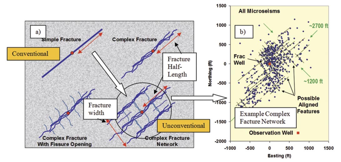
According to Cipolla et al. (2011a), the “ultimate goal of microseismic mapping is to provide insights that link fracture geometry and complexity to well performance, which requires integrating the microseismic interpretation with fracture and reservoir models”. In this work, we emphasize integration of MSMA with RTA and note that both are characterization techniques that can serve as an important precursor for, as well as used iteratively with, fracture and simulation modeling. Proper analysis of both can serve to provide constraints for simulation efforts, which require integration of a wide variety of data sources. Rate-transient analysis provides estimates of effective hydraulic fracture length (low-complexity fractures) or effective fracture network area (complex fracture networks) which can be considered “performance-based” estimates – i.e., these estimates can be used to match well productivity. Microseismic data on the other hand allow for estimates of created fracture half-length or network; comparison of RTA and MSMA estimates can therefore be used to infer what percentage of the fracture length/network is actually effective, allowing for improvements in hydraulic fracture design. The goal is to maximize fracture effectiveness in unconventional reservoirs.

Barree et al. (2005) provided comparisons of hydraulic fracture half-length estimates for low-complexity scenarios derived using multiple techniques, including post-fracture pressure transient analysis, production (rate-transient) analysis and fracture treatment pressure analysis (hydraulic fracture modeling). They also provided insight into the causes of discrepancies observed in estimates from each source. They noted that fracture treatment analysis results in the most optimistic values of fracture halflength, and production data analysis the most pessimistic, but further state that the latter is the most accurate for evaluating the effective flowing fracture half-length. The techniques used for production analysis in the Barree et al. (2005) study utilize time functions (material balance time) that may result in overly pessimistic values for fracture half-length (Clarkson and Beierle, 2011), which could mislead fracture design. No comparisons with microseismic-derived fracture half-length were provided.

In this work, integration of RTA and MSMA is discussed in the context of an overall field development optimization strategy (Figure 2), in which the objective is to determine the appropriate wellbore architecture (vertical versus horizontal, orientation for horizontals), well spacing, completion design (openhole versus cased hole, stage isolation method, frac spacing) and stimulation design (fluid and proppant choices, fluid volumes and pump schedule). RTA, constrained by microseismic interpretations, is used to obtain preliminary estimates of hydraulic fracture and reservoir properties, which are then compared with hydraulic-fracture modeling and serve as a starting point for reservoir simulation. Reservoir simulation and hydraulic fracture modeling sensitivities, combined with economic criteria, are used to optimize field development (see Clarkson et al., 2011a).

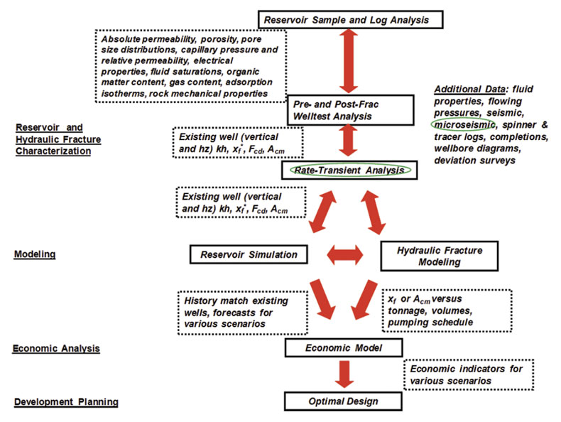
It should be noted that for the case of complex fracturing, new rigorous approaches for simulation and fracture modeling have been developed (i.e. Cipolla et al. 2011b) which also integrate microseismic, but the new modeling techniques require a very complete geological, petrophysical, and geomechanical dataset along with substantial computational effort. Further, these complete data sets will likely only be available during pilot studies, or possibly early development – rigorous modeling of all wells in a full development scenario will likely not be a realistic goal with incomplete datasets. Because production, and in most cases flowing pressure estimates, will be available on all wells, rate-transient analysis can therefore be performed on most wells in the field, given sufficient data quality. It is therefore logical to integrate RTA with MSMA during the piloting phase as a precursor to more rigorous simulation/ hydraulic fracture modeling to a) provide initial constraints on the more rigorous model inputs and b) allow more confident application of RTA to wells where complete datasets are unavailable.

In the following, the concepts of rate-transient analysis and microseismic monitoring and analysis are first discussed, with an emphasis on the former due to familiarity of the geophysicists with the latter. The integration of RTA with MSMA will then be demonstrated for a tight gas (siltstone) reservoir in Western Canada. Finally, the extension of these principles to shale gas reservoirs will be discussed.

1. Concept of Rate-Transient Analysis

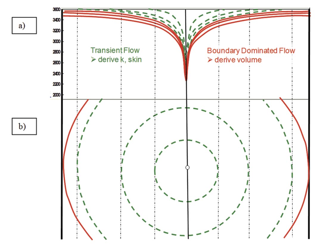
Rate-transient analysis, in the context of unconventional gas reservoirs, involves the interpretation of characteristic flowregimes, which evolve during production of a well, to extract quantitative information about hydraulic fracture and reservoir properties. The procedure and theory for rate-transient analysis is analogous to pressure-transient analysis; in fact, the modern concept of rate-transient analysis is to analyze production data like one would a long-term drawdown test, which is a classic well-test procedure. For constant rate production of a single well, the flowing pressure of the well, which changes during the test, is interpreted using classic well-test analysis concepts. Two primary flow-regimes are typically observed (Figure 3): 1) transient flow, where the pressure transient is propagating away from the well during production and 2) boundary-dominated flow, where all reservoir boundaries have been contacted and the reservoir is now depleting like a tank. Transient flow can be interpreted for hydraulic fracture or reservoir properties, depending on which flow-regimes are observed (discussed below), and boundary-dominated flow can be interpreted to obtain reservoir volume and hydrocarbon-in-place. Because solutions to flow equations used in pressure/rate transient analysis were derived for the case of 1) constant rate or flowing pressure and 2) slightly compressible fluid (water or undersaturated oil), among other simplifying assumptions, several “corrections” are required to reflect 1) changing operating conditions (changing flow rates and flowing pressures) and 2) variable fluid and/or reservoir properties during production. The principal of superposition is used to correct for the former and pseudovariables (pressure and time) are used to correct for the latter. A full discussion of these corrections is beyond the scope of the current study; the reader is referred to texts on pressure transient analysis (ex. Lee, Rollins and Spivey, 2003) for in depth reviews.

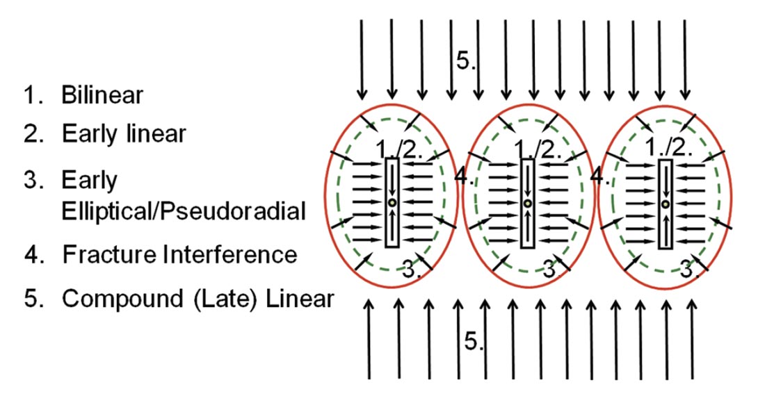
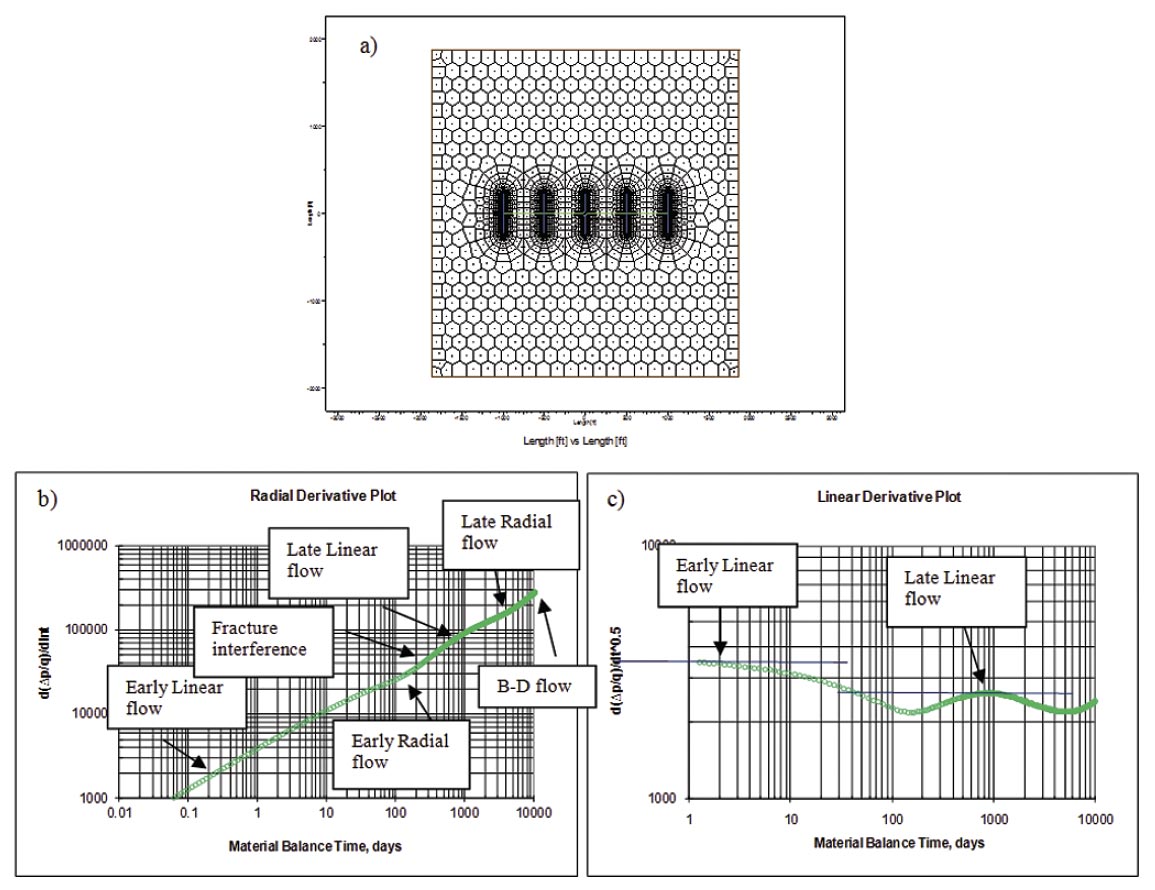
For hydraulically-fractured wells, particularly multi-fractured horizontal wells completed in unconventional gas reservoirs, the sequence of flow-regimes can be much more complex than that shown in Figure 3. For example, the theoretical flow-regime sequence during transient flow for a MFHW (3 stages, wide spacing, assuming planar fracs) completed in a relatively high permeability reservoir is given in Figure 4. The first 3 flow regimes correspond to transient flow between hydraulic fractures, and can be interpreted for hydraulic fracture properties and possibly reservoir permeability (if elliptical or pseudoradial flow is fully developed). Fracture interference then occurs (pressure emanating from each individual fracture “touches” the adjacent fractures). From then on, flow is to the well (ex. compound linear flow) instead of between the fractures.

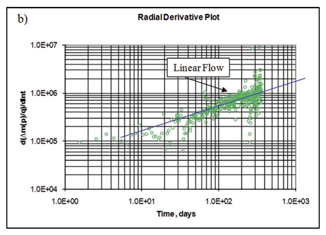
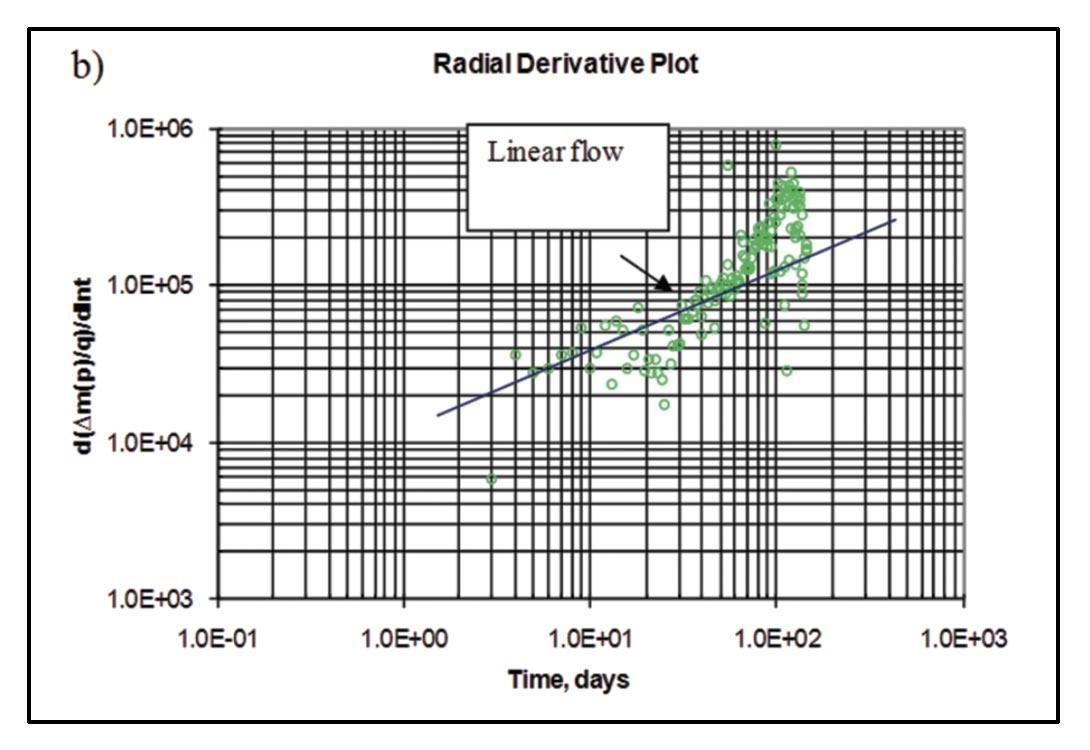
A common way to identify the flow-regimes is to use derivative analysis of the changing flow rate or pressure during time. An example using a simulated multi-fractured horizontal well is provided in Figure 5. The flow-regimes can be identified by characteristic slopes on the derivative plots. For example, linear flow shows up as ½ slope on the radial (semilog) derivative (Figure 5b) and as a zero slope on the linear derivative plot (Figure5c).

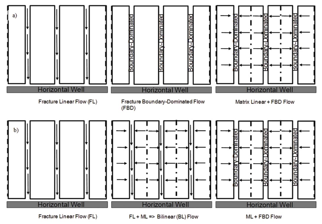
For shale gas reservoirs, where more complex fracturing may be expected (Figure 1), the sequence of flow regimes may be somewhat different than the example shown above (Figure 5); further, the duration and timing of flow regimes could be quite different. An example is provided in Figure 6 from Moghadam et al. (2010), which shows two possible sequences of flow regimes associated with shale gas reservoirs exhibiting transient, dual porosity behavior. Although the induced hydraulic fractures can form a complex fracture network, the matrix blocks have been idealized as slabs in this portrayal.

Of importance to this discussion is what dominant flow regimes may be expected. It is generally believed (ex. Bello 2009) that the dominant transient flow regime in shale gas reservoirs is linear flow from the matrix to the fractures. There could also be a linear flow period associated with linear flow in the hydraulic fractures, but this is generally considered to be short lived, or masked by hydraulic fracture cleanup or skin effects. Further, there may be a linear flow period associated with linear flow from outside the stimulated reservoir volume (outside the idealized fracture network in Figure 6, analogous to compound linear flow in Figure 4) that occurs later in time than the aforementioned linear flow periods.

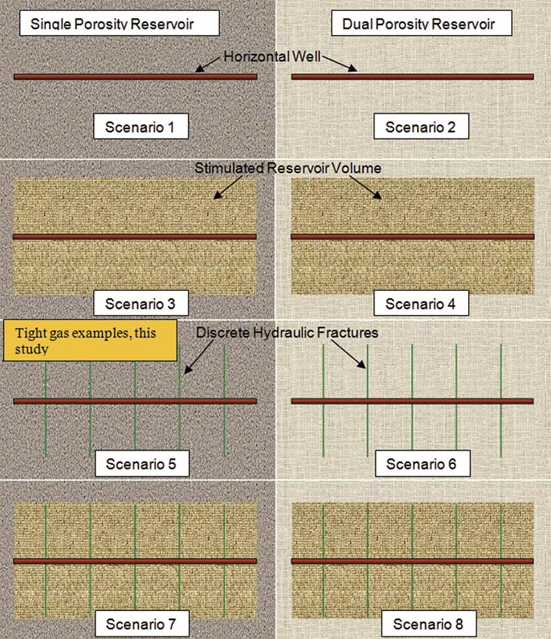
Figures 4 and 6 illustrate the possible sequence of flow regimes for two possible combinations of reservoir behavior and induced hydraulic-fracture geometry, when in fact a wide range in possibilities may occur (Clarkson and Pedersen, 2010). Figure 7 illustrates several combinations that could exist for unconventional gas reservoirs. Scenario 1 illustrates a non-stimulated horizontal well in a single porosity reservoir, which is typically not used to exploit ultra-low permeability shale gas reservoirs, but is still being used for some tight gas and coalbed methane reservoirs. The conceptual model of Scenario 2 may be applicable to non-stimulated horizontal wells in a dual porosity (naturally-fractured) reservoir or a multi-fractured horizontal well where a complex hydraulic fracture network has been created. Some researchers (see Bello and Wattenbarger 2008, Bello 2009) have chosen to represent the induced hydraulic-fracture/stimulated natural-fractures network (or Stimulated Reservoir Volume) as a transient dual porosity reservoir (Figure 6). In the conceptual model of Scenario 3, the SRV is limited to a region immediately around the horizontal well, and the background reservoir is single porosity. Scenario 4 is similar to Scenario 3 except the background reservoir is naturally-fractured (dual porosity). The SRV and background reservoir in Scenario 4 would have different fracture spacing/permeability and fracture porosity. Scenarios 5-8 have the same reservoir characteristics as 1- 4, but with discrete hydraulic fractures which have a different conductivity than the background naturally-fractured reservoir.

The understanding of flow geometries caused by hydraulic fracture geometry and reservoir properties is critically important when interpreting rate-transient/decline characteristics of unconventional gas wells. Once the flow regimes are confidently identified, there are several rate-transient analysis techniques that may be applied to obtain hydraulic fracture/reservoir information from them. These techniques will be discussed next.

2. Rate-Transient Analysis Methods

Rate-transient analysis can be used to derive the following information about the reservoir and the wellbore or fracture geometry:

1. Ultimate recovery (EUR) and Original Gas-In-Place (OGIP) – from boundary-dominated flow data
2. Fracture or matrix permeability, hydraulic fracture half-length and fracture conductivity (see Figure 4 and 5) or contacted matrix surface area (see Figure 6), effective wellbore length – from transient flow data

Rate-transient analysis methods use both production rates and flowing pressures in the analysis to account for variable operating conditions of the wells. For the purposes of this review, we divide production analysis methods into several categories (see Clarkson and Beierle 2011 for in-depth discussion):

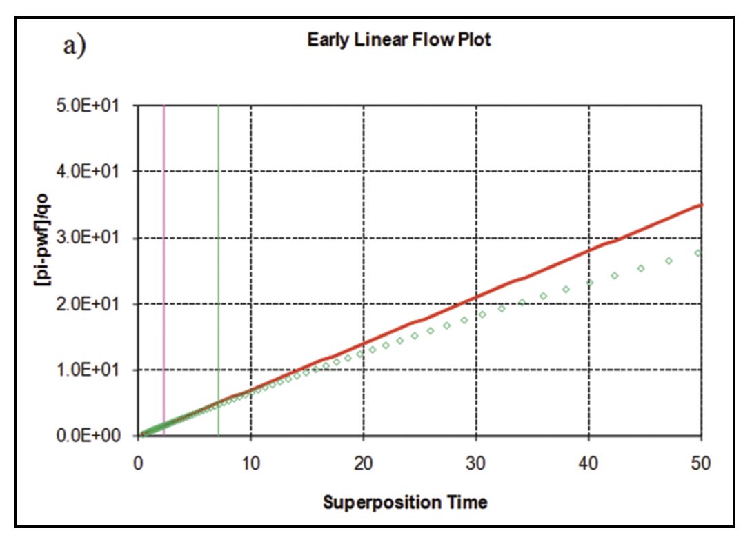
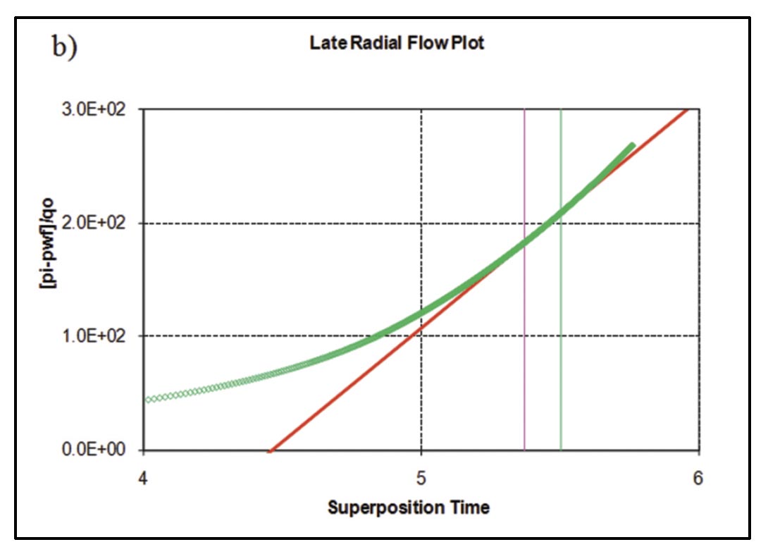
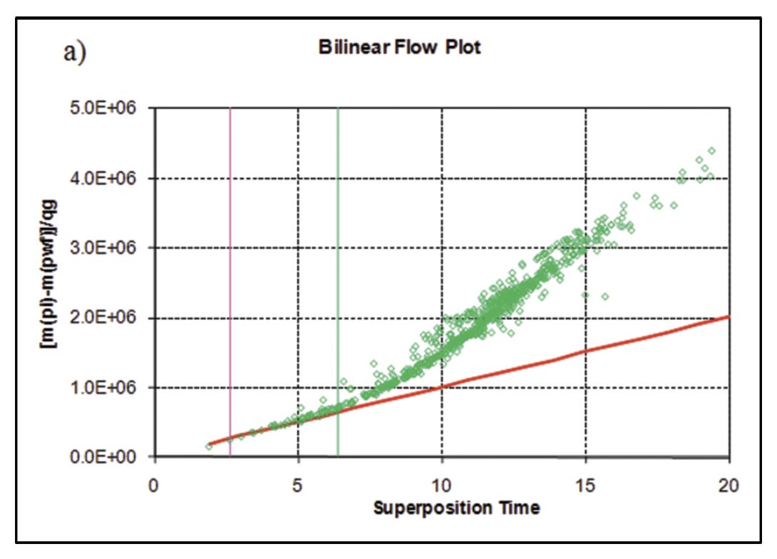
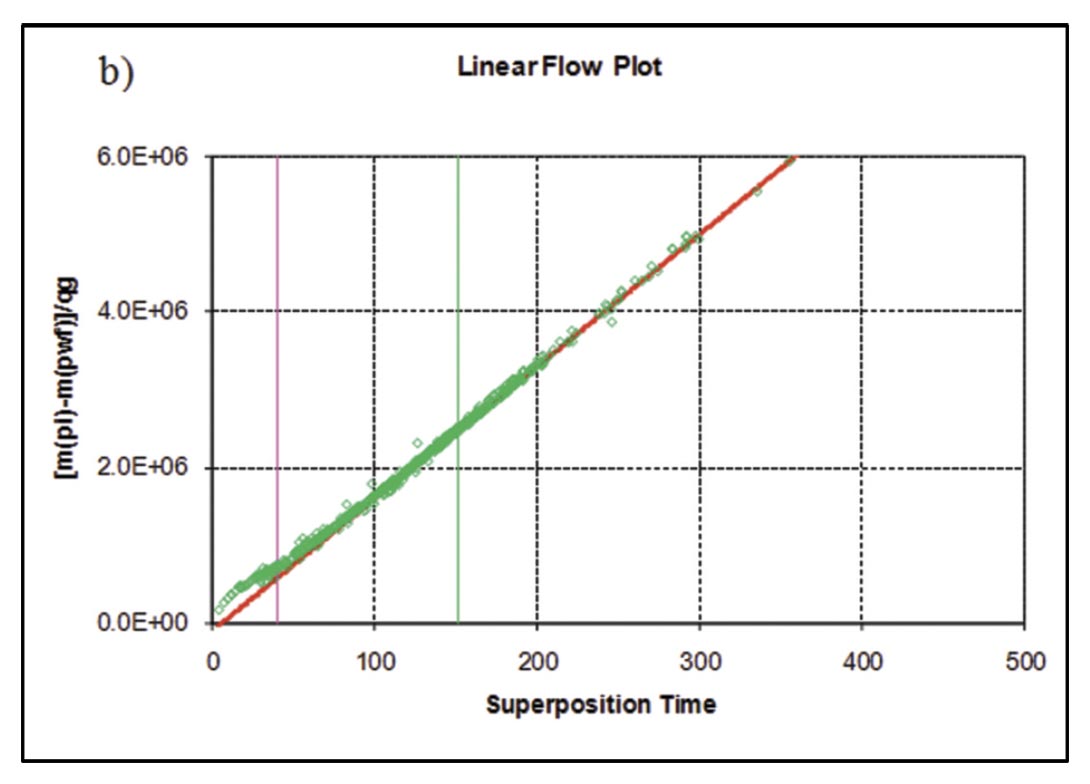
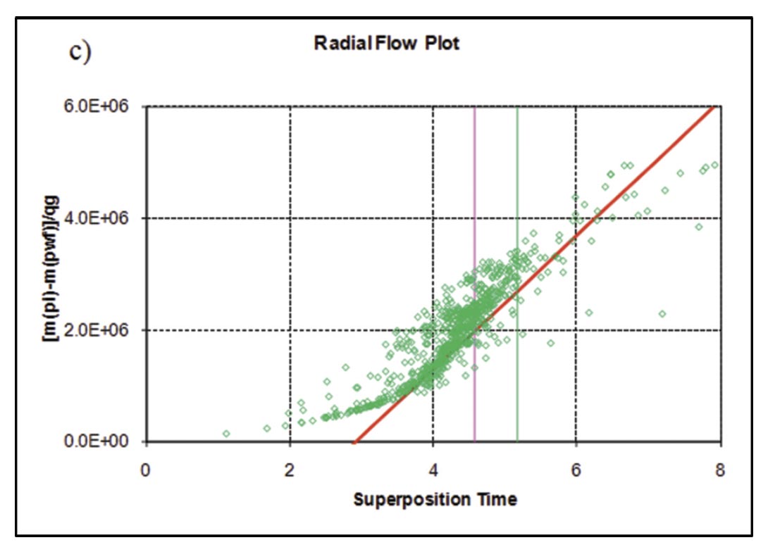
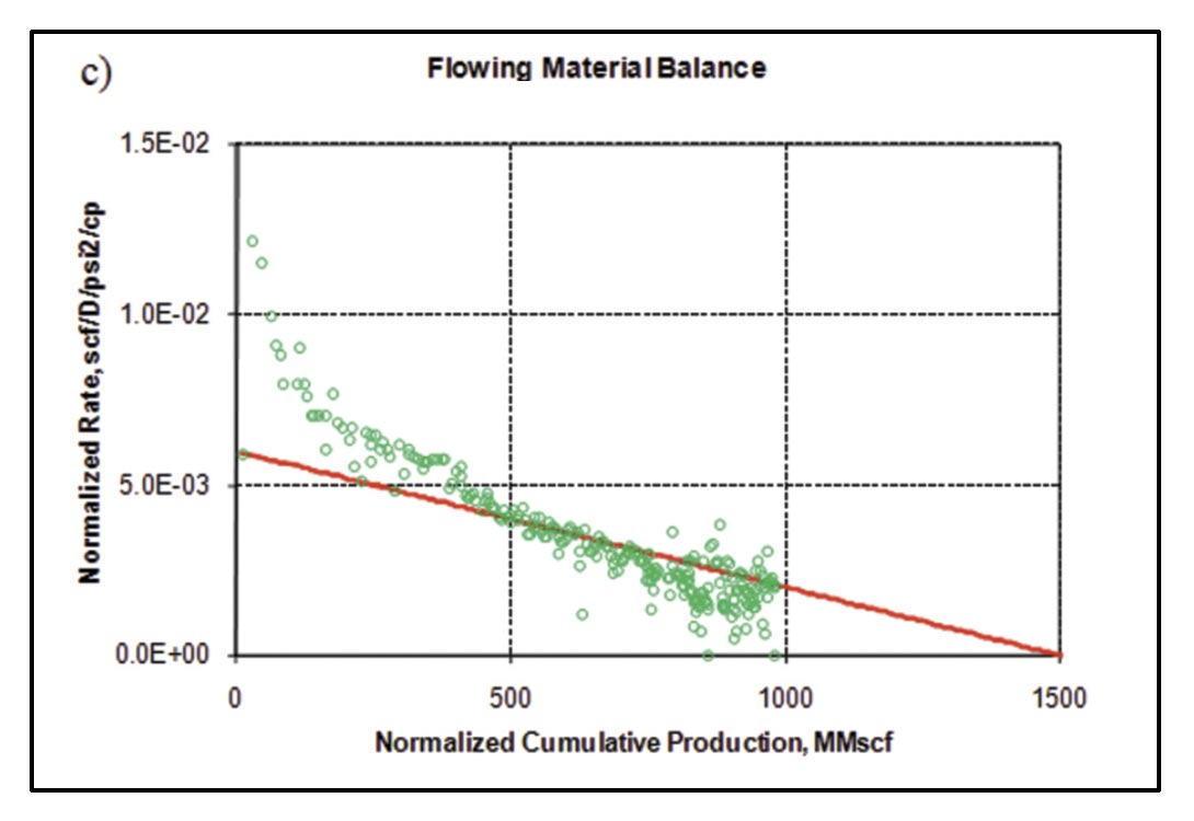
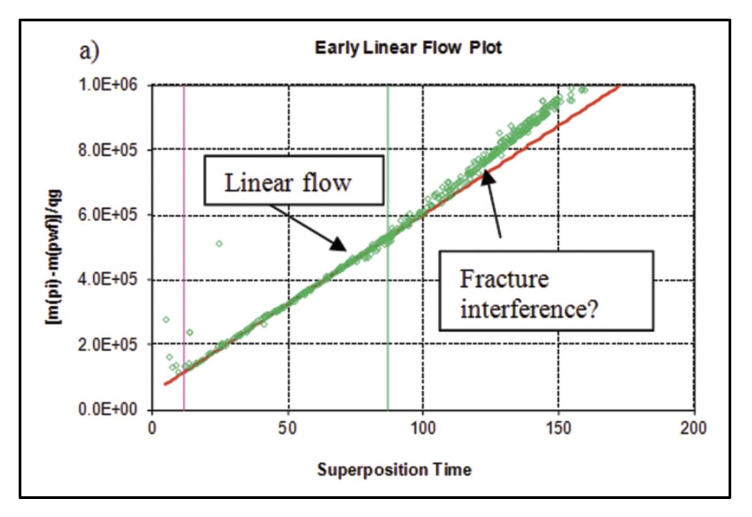
1. Straight-line methods (flow-regime analysis): Once the flow-regimes have been identified using derivative analysis or other log-log diagnostic techniques, the data corresponding to specific flowregimes is analyzed on specialty plots designed to linearize the data set for that flow geometry. For variable operating conditions, superposition time should be used for the x-axis and rate-normalized pressure for the y-axis. If gas is analyzed, pseudotime and pseudopressure should be used to account for variable fluid properties with pressure. Referring to Figures 4 and 5, early linear flow may be analyzed to obtain total effective hydraulic fracture half-length (the sum of all individual fracs emanating from each stage), provided an estimate of permeability. If early bilinear flow is present, an average fracture conductivity for the stages may be obtained, again provided a permeability estimate. Late-linear flow (compound linear flow) may be analyzed to obtain an effective well length, and late radial flow may be analyzed to obtain an estimate of permeability. Lastly, the flowing material balance plot (see Mattar and Anderson, 2005) is a straightline method that can be used to analyze boundary-dominated flow to obtain original gas-in-place. An example analysis of the early linear and late radial flow period for the simulated example case of Figure 5 is shown below (Figure 8).
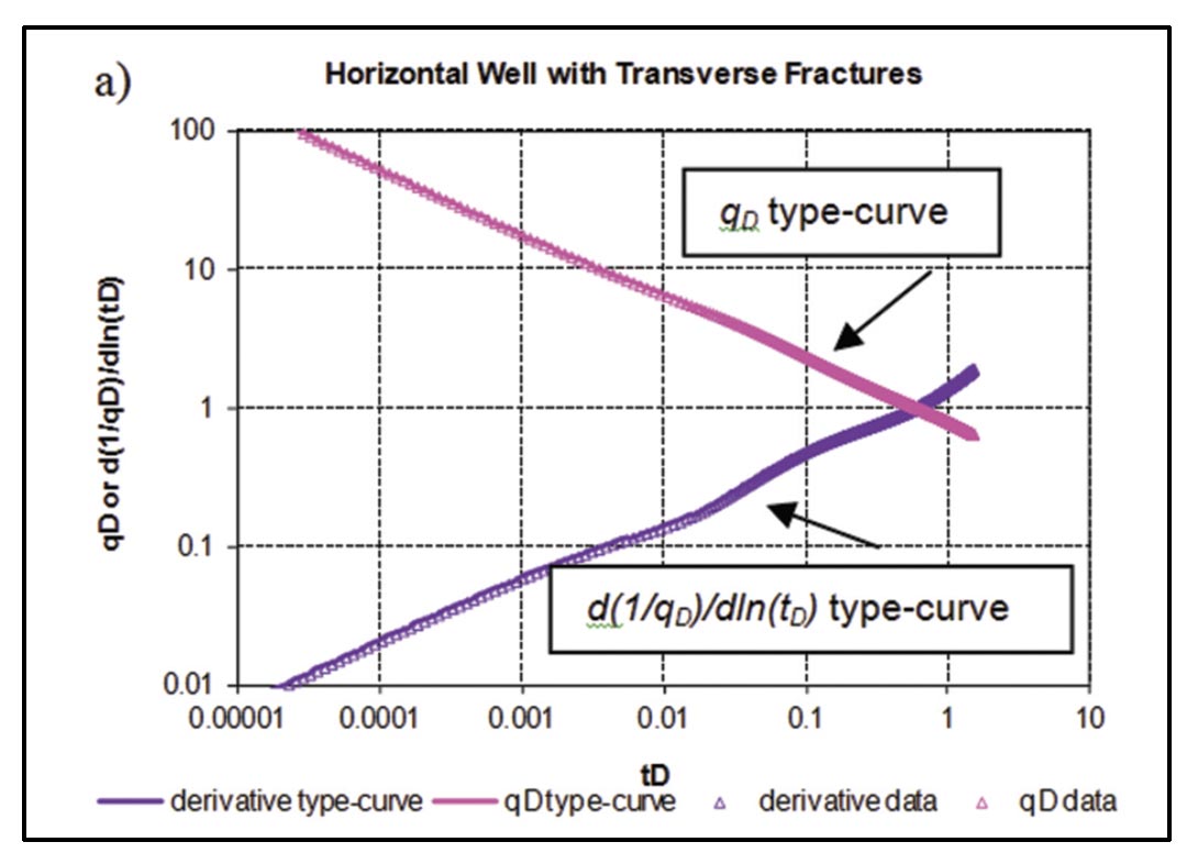
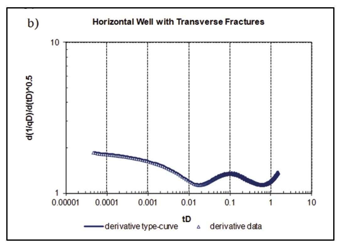
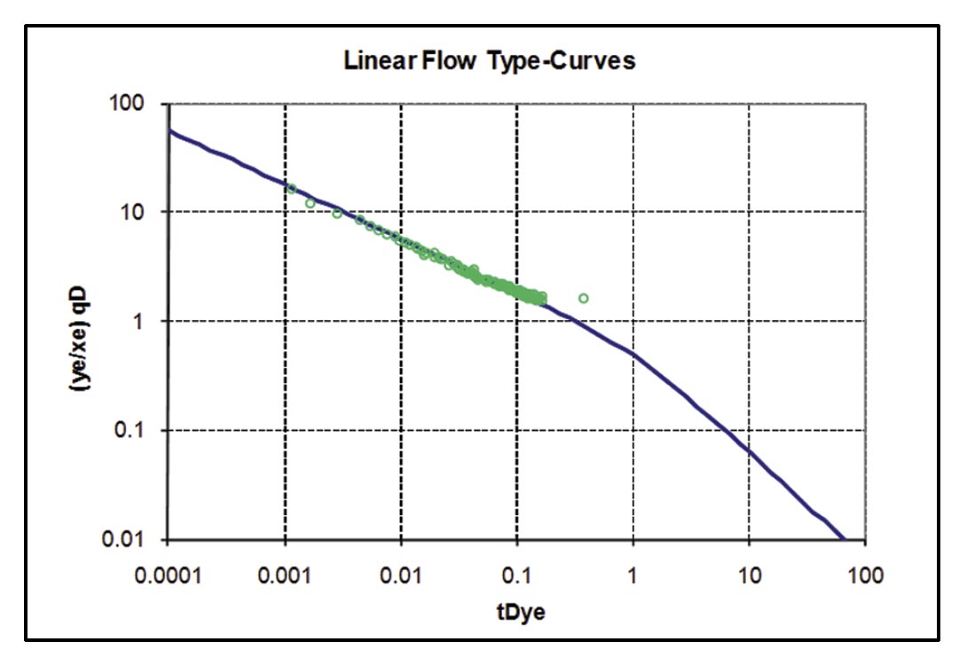
2. Type-curve methods: Type-curve matching involves matching production data (usually adjusted to account for flowing pressure variations) to theoretical/empirical solutions to flow equations that are cast in dimensionless variable format. Reservoir, well-length or stimulation information may be extracted from the match of the data to the dimensionless type-curves, through the definition of the dimensionless variables. An example type-curve match of the simulated data in Figure 5 is given in Figure 9. Note that several type-curve sets are provided corresponding to MFHW Scenario 5 (Figure 7); see full description in Clarkson and Pedersen (2010). The type-curves shown in Figure 9 use traditional definitions of tD and qD – typecurves have also been developed for Scenario 5 using alternative and more robust dimensionless variable definitions (Nobakht et al., 2011a) and for transient dual porosity cases (ex. Moghadam et al., 2010).
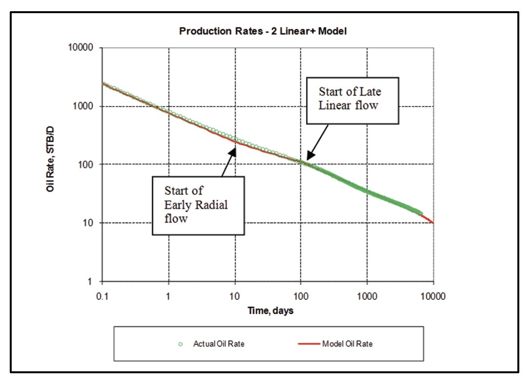
3. Analytical and numerical simulation: Various commercial analytical and numerical simulation tools are available that can be used to analyze single- or multi-well production data. The models are calibrated (a process referred to as “historymatching”) by fitting the model to historical production or pressure (flowing or shut-in) data through adjustment of model inputs. Once an adequate model calibration has been performed, the model may be used to forecast single or multiwell production under a variety of operational and development scenarios. As described by Clarkson and Pedersen (2010), an analytical simulation tool, whose inputs are tied directly to flow-regime analysis outputs, was developed to history-match production data from MFHW corresponding to Scenario 5 (Figure 7). An example match to the numerically- generated data of Figure 5 is shown in Figure 10.

There are also empirical techniques that can be used strictly for forecasting (not for reservoir and hydraulic fracture characterization, which is the subject of this work). Further, there are “hybrid” methods that combine analytical and empirical techniques that can also be used for forecasting (see Nobakht et al., 2010 and Nobakht et al., 2011b).

The example application of RTA provided above (Figure 5) is for the simple case of a MFHW with planar fractures, producing undersaturated oil from a single porosity (homogenous, isotropic) reservoir. RTA can also be applied to the case of shale gas reservoirs, and in particular complex fracturing, as discussed later, but flow-regime id may be challenging (ex. which linear flow period are we seeing?), and complex reservoir behavior may need to be accounted for in the analysis. For example, for shale gas plays, the following reservoir characteristics complicate rate-transient analysis (Clarkson et al., 2011b):

• Low matrix permeability, which causes transient flow periods to last a long period of time
• Dual porosity or dual permeability behavior, due to existence of natural fractures or induced hydraulic fractures (or both)
• Additional reservoir heterogeneities, such as multi-layers (interbedded sand/silt/shale) and lateral heterogeneity
• Stress-dependent permeability, due to a highly compressible fracture pore volume
• Desorption of gas from organic matter in the shale
• Multi-mechanistic (non-Darcy) flow – in shale matrix, caused by gas-slippage along pore wall boundaries and diffusion (see Javadpour 2009), or in the hydraulic fractures due to inertial flow

Recent efforts (Clarkson et al., 2011c, Nobakht et al., 2011c) have demonstrated that desorption, non-static permeability and multi-mechanistic flow can be corrected for in the analysis, by incorporating these properties into pseudopressure/pseudotime variables. With these “corrections”, shale gas data may be analyzed using methods developed for slightly compressible fluids/static reservoir properties. This is an active area of research and the techniques will improve over time.

A workflow for the application of RTA to hydraulically-fractured vertical wells and multi-fractured horizontal wells was provided by Clarkson and Beierle (2011). This workflow involves use of straight-line, type-curve and analytical simulation and is demonstrated later with a tight gas example. A key component of that workflow is the integration of RTA with microseismic to assist with model selection and model calibration.

3. Microseismic Monitoring and Analysis

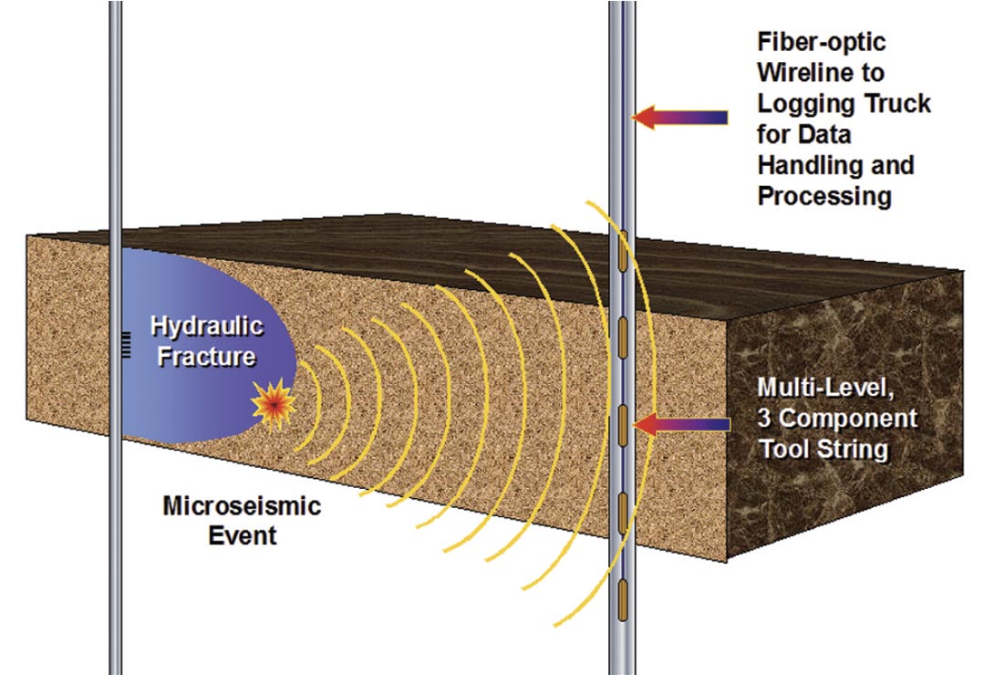
MSMA is increasingly being used as a method to interpret hydraulic fracture growth, and ultimately the geometry of a hydraulic fracture or induced hydraulic fracture network, for unconventional gas reservoirs. According to Warpinski (2009): “microseismic monitoring is the placement of receiver systems in advantageous positions from which small earthquakes (microseisms) induced by some downhole process can be detected and located to provide geometric and behavioral information about the process.” To monitor hydraulic fracture stimulations in vertical wells (Figure 11) an array of three-component geophones is placed in an offset vertical well, at a depth close to the zone being stimulated in the treatment well. Seismic energy associated with microseisms created by hydraulic fracture operations is processed, resulting in placement of the “events” in space (Warpinski, 2009). Similarly, operators have successfully placed geophone arrays in horizontal wells to improve spatial resolution of microseismic events. Ideally both horizontal and vertical wells are used for observation.

According to Cipolla et al. (2011a), microseismic monitoring is the “most widely used technology to measure hydraulic fracture geometry because it provides the most complete picture of hydraulic fracture growth.” Ideally, microseismic data can be interpreted to provide estimates of fracture length, height, azimuth, complexity, and location with respect to exit point from the wellbore; further geologic controls on hydraulic fracture growth (ex. faults) can also be inferred (Cipolla et al., 2011a). The physical processes (i.e. rock failure due to shear) that create microseisms ensure that events are only indirectly related to hydraulic fracture growth. Further, as noted above, MSMA allows for estimates of created fracture half-length or network, and must be integrated with other data and analysis to establish how much of the created fracture network is effective or contributing to flow.

As reviewed by Cipolla et al. (2011a), microseismic mapping involves several steps, including determination of event distance, azimuth and depth. Those authors discuss several possible causes of event location uncertainty and note that uncertainty in event location can cause errors in fracture geometry interpretation, including interpretation of fracture complexity when it does not exist.

Of particular importance to this study is that Cipolla et al. (2011a) integrated microseismic data with fracture modeling, accomplished using both simple approaches and complex hydraulic fracture propagation models, to determine the % of the created fracture area that is propped (i.e. contained proppant) and hence conductive. In the shale gas examples provided by those authors, < 10% (ranging from 3.5 to 7.7 % in the examples provided) of the fracture area is propped at reasonable proppant concentrations. These kinds of studies are important for fracture design optimization because proppant distribution will have an impact on fracture conductivity. It is possible that unpropped fractures will retain some conductivity. However, by analogy to the studies performed by Barree et al. (2005) for tight gas reservoirs, the effective flowing fracture area, as determined by RTA, may be even smaller than the effective propped area determined from hydraulic fracture modeling. The author is unaware of any such comparisons for shale gas reservoirs exhibiting complex fracture geometries.

In the following study, RTA-derived effective half-lengths are compared to microseismic, well-test and hydraulic fracture modeling-derived values for a tight gas reservoir. Although the hydraulic fracture geometries are interpreted to be of lowcomplexity, such comparisons may provide some insight into what to expect for more complex geometries.

4. Example of Integration of RTA and Microseismic for a Tight Gas Reservoir

In a study by Clarkson and Beierle (2011), hydraulically-fractured vertical and horizontal wells were analyzed using rate-transient techniques for a tight gas reservoir in Western Canada. Rate-transient analysis of vertical wells was first performed to establish estimates of reservoir (ex. kh) and hydraulic fracture (effective length and conductivity) properties, prior to analysis of multi-fractured horizontal wells, which were used in later development. The consistency in stimulation treatments for both vertical and horizontal well hydraulic fracturing stages allowed for direct comparison of results. Microseismic data gathered during hydraulic fracturing operations for vertical wells and horizontal wells were used to select models for rate-transient analysis and to determine created versus effective fracture half-lengths.

4.1 Vertical Well Analysis

Vertical wells in the study area were completed in a very consistent way – 2 reservoir intervals were stimulated in 2 stages. Stage treatments typically consisted of pumping 260 gallons of 15% HCl, followed by 70,000 gallons of a polymer-free, water-based stimulation fluid (some breaker required to reduce viscosity before production) with 4% KCL at a rate of ~ 9.5-15 bpm. Approximately 154,000 lb of 20/40 mesh Jordan sand and 22,000 lb of a resin coated ceramic proppant were used.

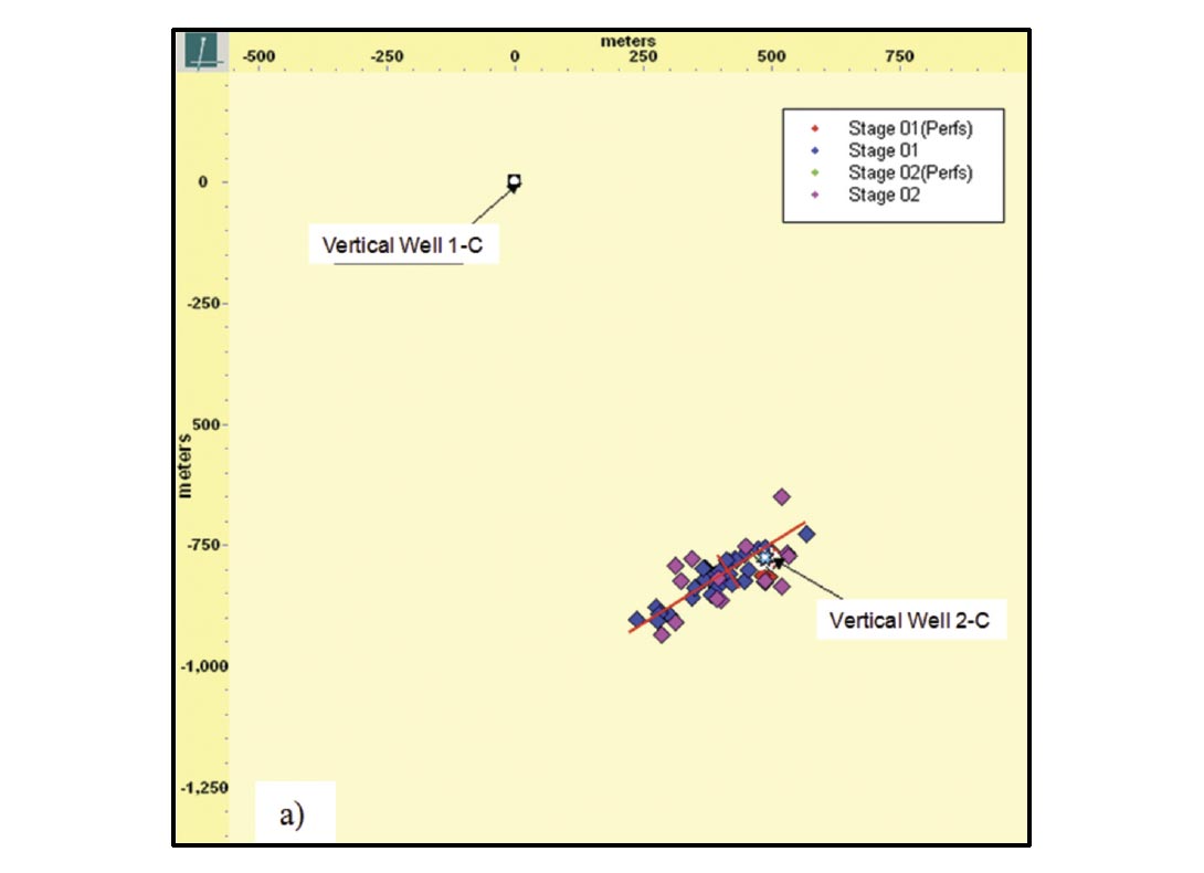
From microseismic analysis, it is believed that the resulting hydraulic fracture geometries for both stages in the vertical wells are of low-complexity (Figure 12). Vertical well 2-C in Figure 12a is for a vertical well that was stimulated with a relatively highrate (60 bpm) slickwater treatment, with much higher fluid volumes than the offset wells. Due to a large distance between the observation well to the treatment well, only a few microseismic events were recorded – the resulting hydraulic fracture geometry is therefore somewhat uncertain. The calculated fracture complexity index (Cipolla et al. 2008) for well 2-C is < 0.2 for stage 1, which according to Cipolla et al. (2011a), is indicative of relatively planar fractures. Stage 2 appears to be of higher complexity.

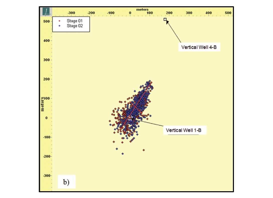
Vertical well 1-B in Figure 12b was stimulated with a more typical low-rate treatment as described above. Due to a more optimal observation well location, more events were recorded in this case. The calculated fracture complexity index for well 1-B is ~ 0.3 for stage 1, suggesting some complexity. Stage 2 appears to be of higher complexity. In this case, some observation well bias is likely. As suggested by Cipolla et al. (2011a), this can lead to azimuthal uncertainty, which in turn can cause the fracture to appear more complex than it is. From analysis of the multi-fractured horizontal wells, in which two observation wells were used (see below), the fractures appear to be less complex than for vertical well 1-B. A planar frac model was therefore assumed for rate-transient analysis of vertical and horizontal wells in the study area.

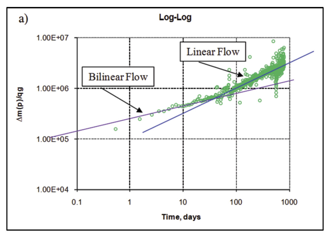
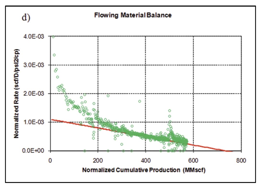
Following the procedure described by Clarkson and Beierle (2011) for rate-transient analysis, flow-regimes for vertical wells in the study area were first identified (Figure 13), followed by flow-regime and type-curve analysis (Figure 14). A log-log diagnostic plot (rate-normalized pseudopressure drop versus time) was used as well as a radial (semi-log) derivative. The diagnostic plot clearly indicates bilinear (1/4 slope) followed by linear flow (1/2 slope), which can be interpreted for fracture conductivity (Figure 14a) and fracture half-length (Figure 14b), respectively, using flow-regime (straight-line) analysis methods, provided a permeability estimate. Radial flow does not appear to be reached, therefore radial flow analysis, assuming the last few data points have entered radial flow will yield an over-estimate of permeability (Figure 14c). Likewise, boundary-dominated flow has not been reached, so the estimate of gas-in-place from the flowing material balance plot will yield a minimum estimate for gas-in-place (Figure 14d).

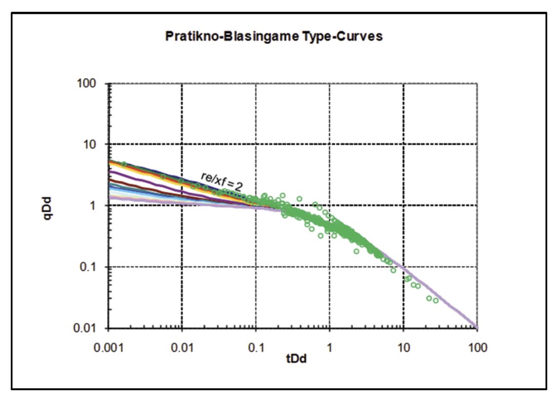
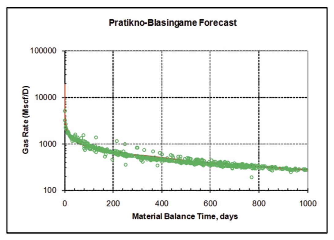
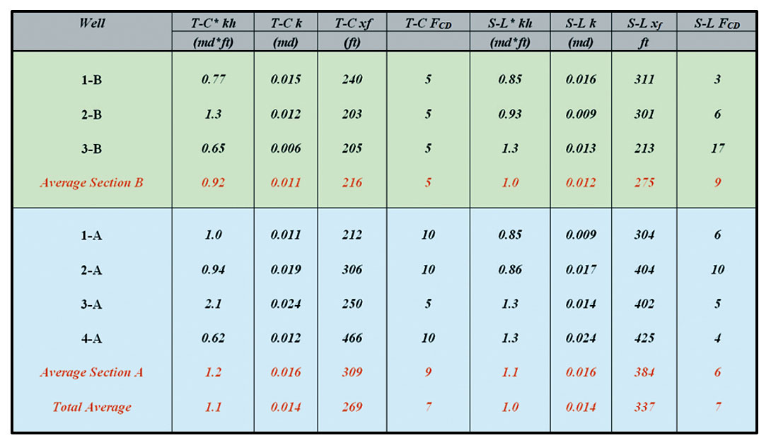
A Pratikno-Blasingame type-curve (Pratikno et al., 2003) match of the same vertical well is shown in Figure 15. These typecurves assume a planar hydraulic fracture geometry, and finiteconductivity fractures. The fracture conductivity obtained from the bilinear flow plot (Figure 14a) was used to guide selection of the type-curves. The resulting fracture half-length obtained from the transient stem match (r_e /x_f = 2) of this well is 212 ft, versus 304 ft obtained from linear flow analysis (Figure 14b). The discrepancy is likely due to the different time functions used in the analysis, as discussed by Clarkson and Beierle (2011); recently Nobakht and Clarkson (2011a,b) provided rigorous corrections to pseudotime to improve analysis. The permeability estimate from the type-curve match is 0.0091 md, versus .011 md from radial flow analysis (Figure 14c).

Multiple vertical wells in the study area were analyzed using this approach, with the results summarized in Table 1. The effective fracture half-lengths from rate-transient analysis average from 269 to 337 ft, depending on whether type-curve or straight-line (flow-regime) analysis methods are used. Of particular interest to this study is how these estimates compare to independent estimates of fracture half-length, including microseismic.

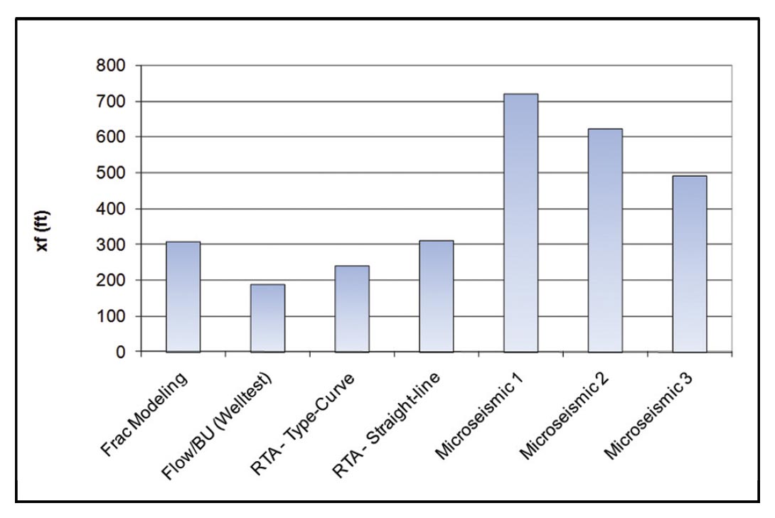
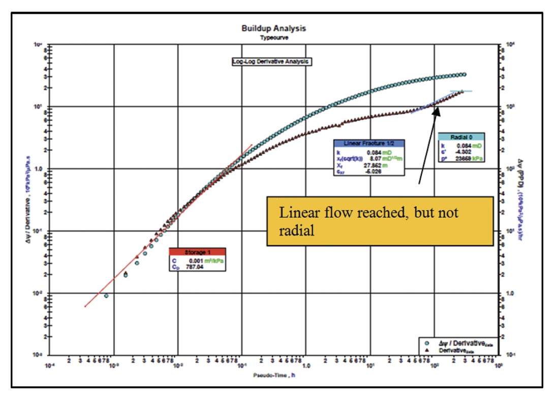
For well vertical 1-B (Figure 12b), estimates of hydraulic fracture half-length were available from rate-transient analysis (Table 1), hydraulic fracture modeling (net pressure analysis), post-stimulation well-testing (flow and buildup analysis) and from microseismic data analysis. A comparison of these estimates is provided in Figure 16. Rate-transient analysis-derived values were obtained using the approach illustrated above – estimates from both type-curve (T-C) and straight-line (S-L) are given. The post-fracture buildup (welltest) analysis is shown in Figure 17 – the test was too short to reach radial flow, but a linear flow period is evident meaning that the hydraulic fracture half-length can be estimated given a permeability estimate. Using the RTA-derived permeability estimate, the calculated fracture half-length from the buildup test is approximately 200 ft, which is smaller than, but in reasonable agreement with, the RTA type-curve estimate. Hydraulic-fracture modeling was performed using a commercial hydraulic fracture model, and hydraulic fracture treatment data collected during the frac job – estimates of propped fracture halflength for both frac stages was provided, and the average is given in Figure 16. The propped fracture half-length is very consistent with the straight-line (RTA-derived) values of effective halflength, but somewhat larger than the type-curve (RTA-derived) values. The difference between effective flowing and static propped half-length is small in this case, but the RTA-derived fracture conductivities are much smaller than those from hydraulic fracture simulation – this is to be expected as fracture conductivity while the well is flowing is expected to be reduced due to multi-phase flow, fracture conductivity degradation etc.

Lastly, note that there are three estimates of created fracture halflength from the microseismic data. Three different vendor companies were asked to process the raw data, and these values represent the estimates from each company. The differences, which are substantial, are related to different processing procedures. In all cases, the microseismic-derived values are substantially larger than well-test, frac model or RTA-derived values. This is due to the fact that microseismic data, while providing an estimate of created halflength (subject to processing uncertainty), does not provide an estimate of effective fracture half-length. The well-test, frac-modeling and RTA-derived values appear to be in reasonable agreement, but are significantly different than microseismic-derived values, suggesting that a substantial portion of the created fracture is nonconductive. Further, RTA suggests that the effective portion of the fracture is of relatively low conductivity.

4.2 Horizontal Well Analysis

As with vertical wells, several horizontal wells in the study area were completed in a very consistent way. An example analysis is provided for the longest-producing well in the study area (horizontal well 1-B), which was completed in 4 stages (openhole, with swell-packers for isolation individual). Stage treatments consisted of pumping ~ 80,000 gallons of the same water-based stimulation fluid as the vertical wells, but at a rate of ~ 25 bpm. Approximately 220,000 lb of proppant (sand) were pumped per stage. The per stage stimulation treatments in this well are similar to the individual stages pumped in offset vertical wells, although with slightly larger fluid volumes and sand amounts. The frac half-lengths and conductivities derived from vertical well analysis (Table 1) therefore provide a reasonable benchmark for horizontal well analysis.

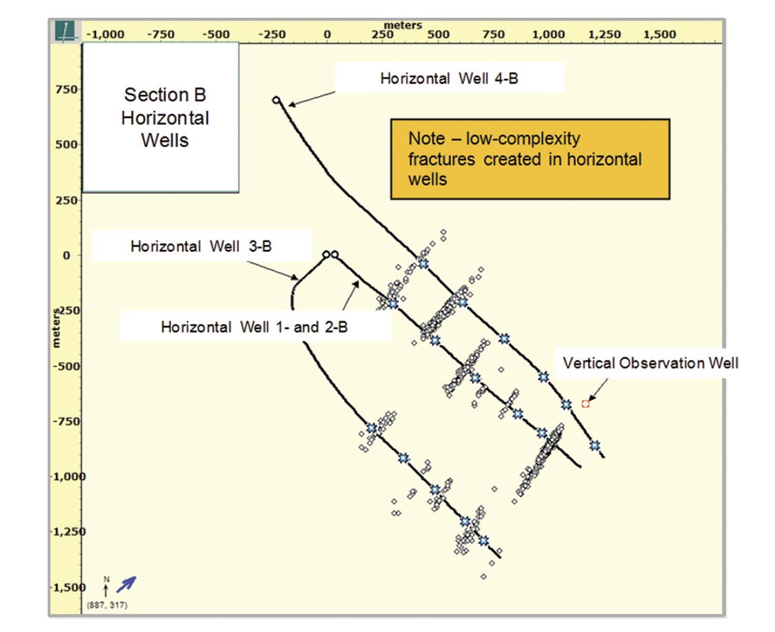
Although microseismic data for horizontal well 1-B were not collected (it served as an observation well), the interpreted microseismic data for offset horizontal wells in the same section suggest low-complexity, if not planar, fractures (Figure 18). Both a horizontal and vertical observation well was used for observation, and dual array processing resulted in a very good dataset. Generally, only one hydraulic fracture appears to exist per stage. The hydraulic fractures are oriented in a NE-SW direction, in agreement with the maximum in-situ horizontal stress direction in this portion of the Western Canadian Sedimentary Basin. A planar hydraulic fracture model was therefore selected for RTA of horizontal well 1-B, and the created half-lengths in offset wells served as a constraint for interpretation.

Following the analysis procedure of Clarkson and Beierle (2011) for rate-transient analysis of multi-fractured horizontal wells, flowregimes for vertical wells in the study area were first identified (Figure 19), followed by flow-regime analysis (Figure 20). The loglog diagnostic plot (Figure 19a) appears to suggest bilinear flow followed by linear flow, whereas the derivative is less clear (the derivative tends to amplify noise in the data). It is possible that the early “bilinear” flow period is related to cleanup of hydraulic fracturing fluids or flow convergence to the well, and not necessarily finite conductivity fracture behavior. At late time, there may be an indication of hydraulic-fracture interference, as evidenced by deviation from ½ slope on the flow-regime analysis plots.

The bilinear flow analysis in Figure 20a provides a “pseudo-fracture conductivity” as it is not clear that the well exhibits a true bilinear flow period. The conductivity value (14 md*ft) is however consistent with values obtained from offset vertical wells. Because an accurate estimate of permeability cannot be obtained from this analysis (late radial flow was not reached), a value of .01 md is assumed, which is consistent with offset vertical well analysis. Although not shown, analysis of the last few datapoints using early radial flow analysis, expected to yield nkh (where n = number of stages), yields a permeability of .015 md, which is in reasonable agreement with the vertical wells. The total effective fracture half-length (sum of individual fracture stage half-lengths) from early linear flow analysis (Figure 20b) is estimated to be 1094 ft; assuming 4 individual hydraulic fractures resulted from the 4-stage completion, the estimated average per-frac effective half-length of ~ 275 ft. This number compares favorably to the 216 ft and 275 ft average xf from Section B vertical well type-curve and straight-line analysis, respectively (Table 1). Given that individual stage fracture treatments were similar in horizontal and vertical wells, the consistency of the extracted hydraulic fracture properties between horizontal wells and vertical wells is important for validation of the approach. In the paper by Clarkson and Beierle (2011), production log data was used to estimate individual fracture stage half-lengths, constrained by the total half-length of 1094 ft.

Fitting the last few data points on the flowing material balance plot (Figure 20c) yields a drainage area of ~ 33 acres, which is slightly larger than the area defined by the last 2 stages and the width of the reservoir defined by the average fracture length (27 acres), which intuitively makes sense as the fractures appear to have started to interfere.

Lastly, type-curve analysis was performed to confirm the hydraulic fracture half-length estimates from straight-line analysis (Figure 21). In this case, no transitional flow regimes (early elliptical or radial) were evident, so the linear flow type-curves of Wattenbarger et al. (1998) were used to match the data, after correction for apparent skin effects (Nobakht and Mattar, 2010).

5. Discussion

As illustrated above using a tight gas example, microseismic data is of importance for both assisting with RTA model selection, and allowing for comparisons of created versus effective hydraulic fracture half-lengths. The latter will factor into completion design. The integration of these two techniques also serves as an important pre-cursor for rigorous reservoir simulation (Figure 2).

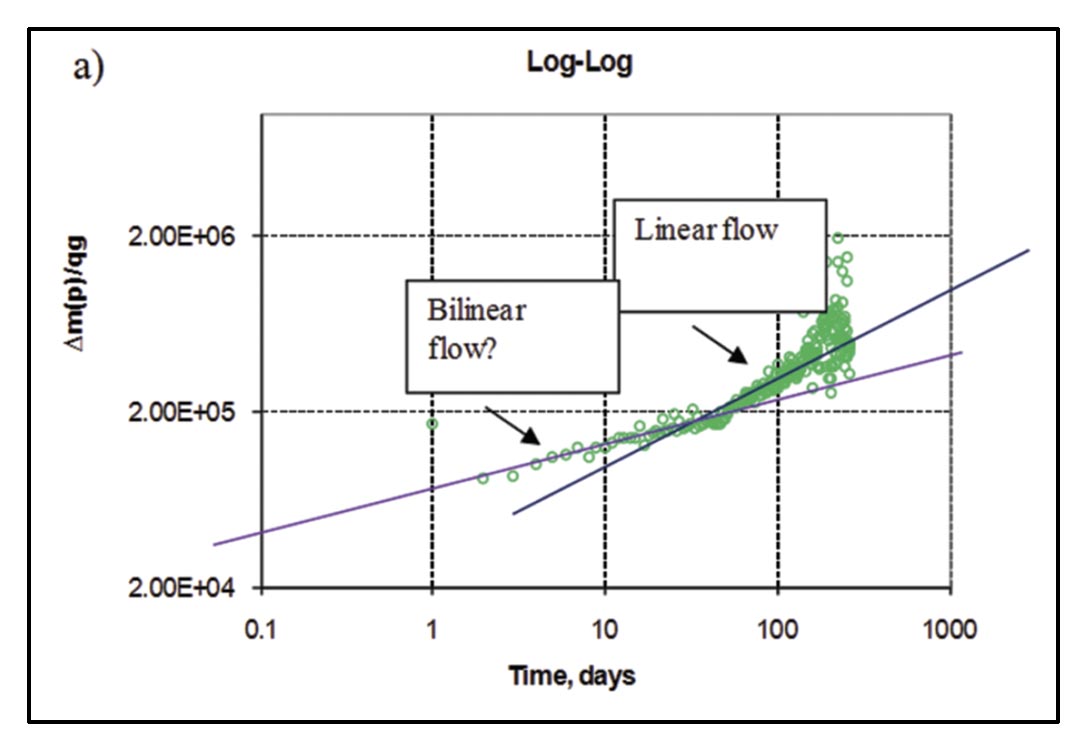
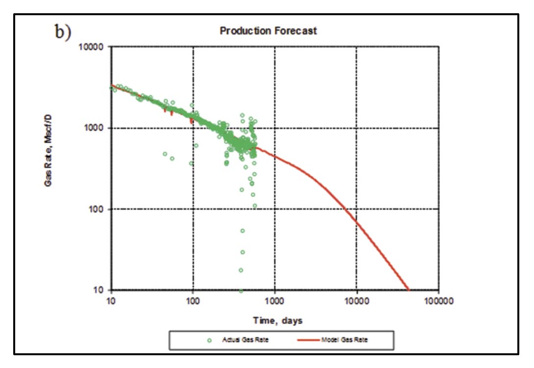
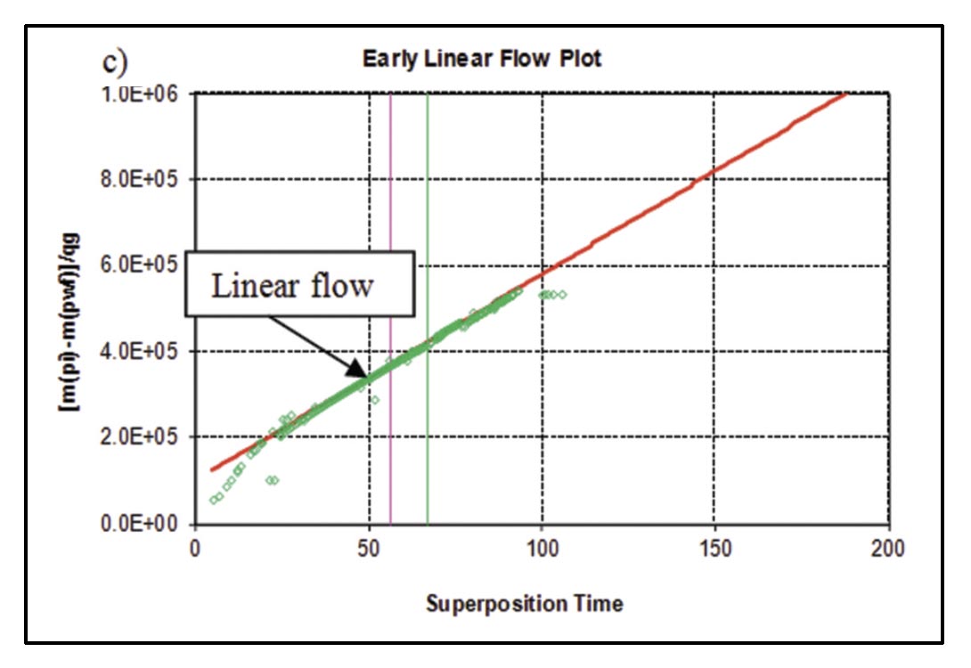
For shale gas reservoirs, an analogous work flow can be followed, but in this case (if complex hydraulic fracture networks are created), it is the matrix surface area contacted by the hydraulic fracture that should be compared between RTA and microseismic data. Rate-transient analysis was performed on two multi-fractured horizontal shale gas wells in two different U.S. shale gas plays. Following a similar process as described above for the tight gas example, flow-regimes were first identified, followed by flow-regime analysis, type-curve analysis and analytical model forecasting. For the two shale gas wells, only the linear flow analysis (Figure 22 a, c) and forecast (Figure 22 b, c) are given.

For shale gas well 1 (Figure 22 a, b), linear flow is followed by an apparent fracture interference (Figure 22a), possibly indicating boundary dominated flow within the stimulated reservoir volume. Assuming that this linear flow period corresponds to matrix linear flow (Figure 6), it can be analyzed to obtain √kA_cm, where A_cm is contacted matrix surface area from which A_cm may be estimated if (matrix) permeability is known. Note for the tight gas example above, we obtained √kx_f from linear flow analysis. In this example, assuming a matrix permeability of 100 nanodarcies, A_cm is ~ 3 x 10⁶ ft². Assuming boundary dominated flow was reached, flowing material balance can be used to obtain an estimate of gas-in-place associated with the SRV. The forecasting procedure described by Williams-Kovacs and Clarkson (2011) was used to generate the forecast in Figure 22b.

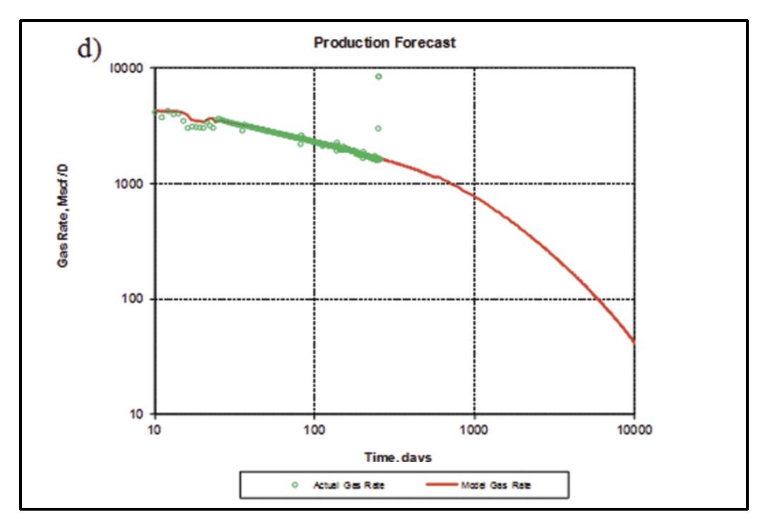
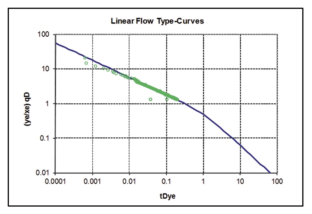
For shale gas well 2 (Figure 22 c, d), only linear flow is apparent. In this case, again assuming the linear flow period is matrix linear flow and a matrix permeability of 100 nanodarcies, A_cm is ~ 5 x 10⁶ ft². The estimate of A_cm was confirmed with a type-curve match, after correction for skin effects (Figure 23). There is no apparent boundary dominated flow, so a conservative forecast is generated by assuming that the well will enter boundary-dominated flow immediately after the linear flow period (Figure 22d). An approximate SRV size can be calculated by using the perforated length of the well and the estimated fracture half-length (per frac) from linear flow analysis – this will result in a larger drainage area and more aggressive forecast. The Acm estimates provided here are consistent with estimates from other authors for shale gas wells (ex. Al-Ahmadi et al., 2010).

Unfortunately, no microseismic data were available for these wells. However, in the work of Cipolla et al. (2011a), who performed microseismic analysis and hydraulic fracture modeling for Barnett Shale well examples, an estimate of the percentage of the fracture area generated by the hydraulic fracture network that was propped was provided. For the two examples given by those authors, this percentage was 7.7 and 3.8 %.

Assuming that the effective flowing surface area is smaller still, this would mean that the estimates of Acm provided above would be much smaller (assuming < 10%, perhaps < 1% in some cases) than that estimated from microseismic analysis. In our examples, the created surface area based on microseismic analysis could be on the order of 10⁷ or 10⁸ ft². Such an analysis would suggest that there is much room for improvement in developing a larger % of effective surface area for shale gas wells.

Another useful application of microseismic data for shale gas wells is for reserve estimates. For shale gas well 1 above, for example, a reasonable lower bound for reserves can be provided if boundary-dominated flow was truly reached and the well is starting to deplete the SRV (Figure 22b). It is expected that the gas volume associated with the stimulated reservoir volume will be less than that associated with the physical well spacing – it is possible that late in time, flow could be contributed from outside the SRV, and hence assuming that drainage is restricted to the SRV could be conservative. A reasonable range of reserve estimates could then be provided by forecasting using a drainage area corresponding to the apparent boundary-dominated flow for this well (low side), and for the well-spacing (high side).

However, intermediate estimates can also be provided by calculating the drainage volume (and conversion to a corresponding drainage area) corresponding with various SRV estimates. Cipolla et al. (2011a) noted that SRV estimates from microseismic are sensitive to data processing. Uncertainty analysis associated with microseismic processing will in turn provide an estimate of SRV uncertainty, which in turn can be used to provide a range in drainage volumes used in forecasting.

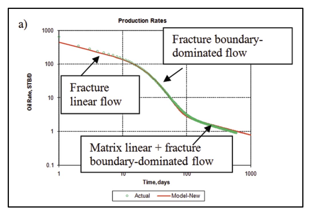
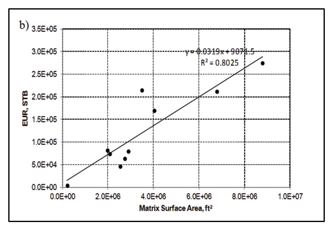
One final useful application of combined RTA and microseismic is for exploration. In a recent paper by Clarkson and Pedersen (2011), vertical wells from a naturally-fractured shale oil play (in Second White Speckled Shale Formation) were analyzed using rate-transient analysis methods. Some of the wells exhibited behavior analogous to Figure 6a, a theoretical flow rate signature for which is shown in Figure 24a (see Clarkson and Pedersen, 2011 for field examples). The late-time matrix linear flow was analyzed and related to estimated ultimate recovery (Figure 24b) for several vertical wells in the play. As discussed in Clarkson and Pedersen (2011), in areas of the play that have an absence of natural fractures, plots like Figure 24b can be used to determine how much matrix surface area must be generated by hydraulic fracture treatments in multi-fractured horizontal wells to meet a reserve hurdle. Of course this is the “effective” area that must be generated, and assumes hydraulic fracture properties would be similar to natural fracture properties, and that such a fracture network can be created, which is uncertain for this play. Further, the effective matrix surface area will not be equal to that generated. Once a pilot test is performed using multi-fractured horizontal wells, hydraulic fracture modeling would be necessary to establish how much surface area would be generated during the hydraulic fracture treatment, and microseismic data would be necessary to calibrate the fracture models, analogous to what has been suggested by Cipolla et al. (2011b). The resulting “created” hydraulic fracture surface area could then be related to “effective” established from production data.

6. Conclusions

The combination of rate-transient analysis with microseismic data is a powerful new approach for optimizing development of unconventional gas and oil plays. Rate-transient analysis is inherently limited to simple models, but utilizes data commonly gathered during field development; more rigorous approaches for characterizing hydraulic fracture properties of unconventional reservoirs are now available (see Cipolla et al. 2011b, Meyer and Buzan, 2011), but require much more data and are computationally intensive. In this work, it is suggested that ratetransient analysis be combined with microseismic data gathering and analysis to provide early estimates of hydraulic and reservoir properties, which in turn can be used as a starting point for more rigorous simulation efforts. Moreover, this “calibration” exercise will prove useful for future well analysis where microseismic and other data required for rigorous frac modeling are not available (i.e. most of the wells in a developed field). Improvements to RTA, as well as MSMA, as applied to unconventional reservoirs, are increasing rapidly. Their combined usage will prove important for future exploration and development applications.

Acknowledgements

The author would like to acknowledge Encana for support of his Chair position in Unconventional Gas at the University of Calgary, Department of Geoscience. He also acknowledges the contributions of his students, in particular Morteza Nobakht and Jesse Williams-Kovacs, who have contributed greatly to the understanding of unconventional rate-transient analysis. Finally, Dave Eaton is thanked for his fruitful discussions on the combination of RTA and MSMA.