How much can I stretch and squeeze?

Well to seismic ties is a fundamental step in seismic interpretation. It relates subsurface measurements obtained at a wellbore measured in depth and seismic data measured in time. A time-depth relationship is typically computed by integrating the slowness function measured at a wellbore. Mis-ties are often present and adjustments to the time-depth relationship are typically fine-tuned by stretching and squeezing of the well logs. However, the validity of stretching and squeezing is sometimes questioned and the question of how much stretching and squeezing is acceptable remains a topic of debate.

In this study, we investigate the idea of using a Backus averaged well log that accounts for dispersion resulting from layer induced long wave elastic attenuation to compute a time-depth relationship. We review the theory to compute a local Q function that results in both positive and negative Q values, which imply that a mandatory stretch and squeeze is required when dispersion is present. We illustrate with an example from Western Canada where the presence of low velocity coals results in large errors in the well to seismic tie. We show that these mis-ties can be reduced by using a Backus averaged well log to compute the time-depth relationship, which accounts for velocity differences between the logging and seismic frequencies. In addition, the ratio of the logging and seismic velocities provides an indication of how much stretching and squeezing is justifiable.

Introduction

Well to seismic ties are fundamental in seismic interpretation as it provides the link between subsurface properties measured directly at a wellbore and the remotely sensed data obtained through seismic sounding. Well logs measured in depth and seismic data measured in time require a time-depth relationship to facilitate the conversion between the two different measurement domains. This could be achieved through a checkshot obtained by vertical seismic profiling (VSP) or the integration of the slowness function obtained by acoustic logging, where differences between the two methods were discussed by Gretener (1961). As checkshots from a VSP are not always available, a time-depth relationship is typically computed using the sonic measurements obtained through well logging.

The well to seismic ties can vary in quality and any mis-ties are typically fine-tuned by stretching and squeezing the well logs to adjust the time-depth relationship. Numerous justifications can be made regarding the validity of stretching and squeezing. These include measurement errors in the well logs and dispersion effects arising from differences in the measurement frequencies, where the seismic bandwidth is typically on the order of 100 Hz and logging frequencies are in the kilohertz range. Although these are valid reasons for manually adjusting the time-depth relationship, many practitioners still struggle with the idea of applying these seemingly arbitrary corrections. Moreover, the question of how much stretching and squeezing is justifiable presents another major hurdle in our quest for an improved well to seismic tie.

In the following, we review the theory as presented by Liner (2014) to compute a local Q function arising from layer induced long wave elastic attenuation. Subsequently, we show that the well to seismic tie can be improved by using a Backus averaged well log to compute the time-depth relationship.

Local Q attenuation

The propagation of seismic waves in a horizontally layered earth results in an apparent attenuation of the seismic energy that is constant Q in nature (Liner, 2014). This attenuation can be related to dispersion through the exact relationship given by Kjartansson (1979),

where V(f) is the velocity corresponding to frequency f, V₀ is the reference velocity corresponding to reference frequency f0 and Q is the quality factor. Equation 1 suggests that a finite Q will result in different frequencies travelling at different velocities. Therefore, with the assumption that we have a constant Q earth, the velocities corresponding to the logging frequencies and seismic frequencies are different and are related through equation 1.

Furthermore, Liner (2014) argues that Backus averaging (1962) can be used to determine the associated dispersion. Because the seismic frequencies are much lower than logging frequencies, the rapidly varying substructure at smaller length scales relative to the seismic wavelength will not be seen by the seismic waves. Backus averaging of the well log velocities then yields the velocity of the effective medium as seen by the seismic waves. Equation 1 can be rearranged to solve for Q as

where λ is the logging depth interval and λ₀ is the Backus averaging length. V and V₀ then represent the velocity as measured by well logging and the Backus averaged well log, respectively. In equation 2, the wavelength is used instead of frequency, following Liner’s argument that the wavelength is the more natural domain of Backus averaging. Equation 2 yields a Q function that describes the local attenuation behavior. A key consequence of Liner’s results is that in addition to the more familiar positive Q, where high frequencies travel faster than low frequencies, local negative Q is also possible, which implies that high frequencies travel slower than low frequencies. In the context of traveltime differences between logging and seismic frequencies, this implies that zones of positive Q require stretching and zones of negative Q require squeezing of the well logs.

Now consider the two-way traveltime given by

where s(z) represents the slowness as a function of depth, z. As mentioned above, t is typically computed using well log measurements and therefore, represents the traveltime associated with the logging frequencies. However, for our well to seismic ties, we are interested in the traveltime associated with the seismic frequencies. Therefore, the s(z) used to compute the traveltime function should be the Backus averaged slowness.

Example

To demonstrate the effects of using a Backus averaged well log to compute the time-depth relationship, we illustrate with an example from Western Canada where the presence of low velocity coals results in large errors in the well to seismic tie. Our target interval is the Glauconite and Ostracod formations in the Manville group, which is overlain by the Top Manville and Medicine River coals. These low velocity coal zones generate a number of complex wave propagation phenomena including multiple generation, transmission filtering (Coulombe and Bird, 1996) and traveltime effects that result in exploration challenges in the underlying formations. In this study, we are interested in the traveltime effects and the associated time-depth errors in the well to seismic tie.

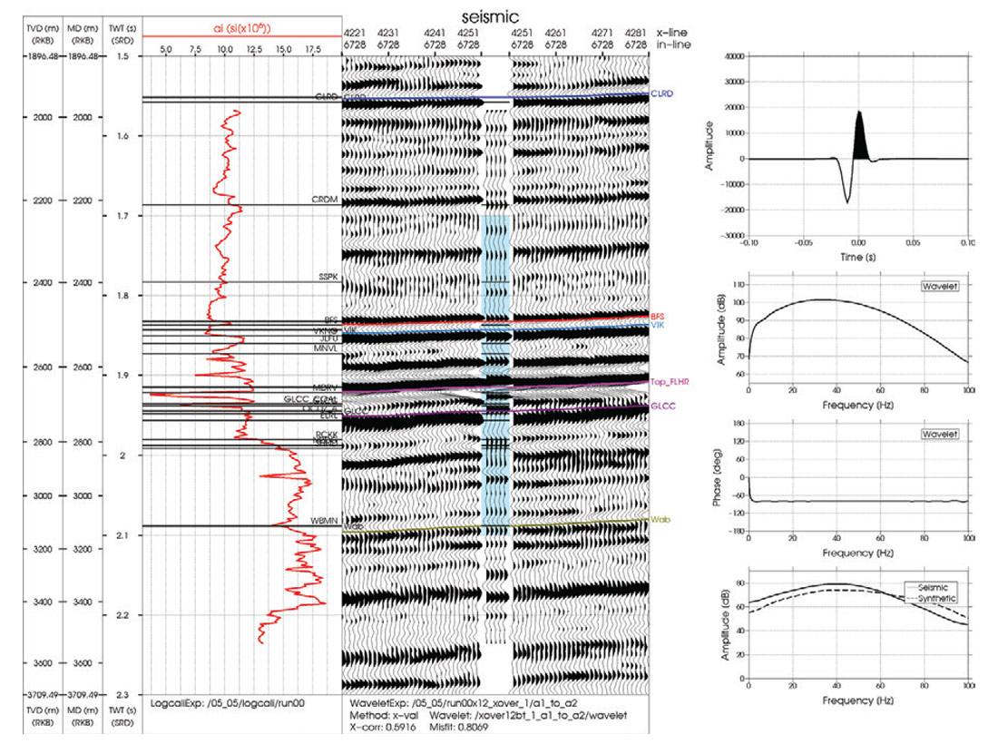
Figure 1 shows the well to seismic tie using a time-depth relationship computed by integrating the well log slowness. The panels from left to right show the acoustic impedance log, seismic section with synthetic insert and the wavelet with its corresponding spectral representations. The coal zones begin just after 1.9 s and are identified by the low acoustic impedance intervals. Note the poor tie in the vicinity of the coals where we have a correlation coefficient of 0.59 in the time window 1.7 s to 2.1 s. The synthetic seismogram would require a large stretch around the coals to visually correct for the traveltime differences.

Next, we investigate the local Q attenuation concept as presented by Liner (2014) for computing a time-depth relationship. Here, our depth sampling interval for the well logs is 0.1524 m and we use an averaging length of 90 m, which corresponds to a maximum frequency of approximately 70 Hz using the relationship, f_max= V_max / λ_min. Figure 2 shows the original logging and Backus averaged velocities and the corresponding local attenuation function defined as the inverse of Q. The local attenuation curve exhibits both positive and negative values, and as mentioned above, results in high frequencies (logging) travelling both faster and slower than low frequencies (seismic). Consequently, stretching and squeezing is required for a proper calibration of the time-depth relationship between the well log and seismic. In Figure 2, it can be seen that at the coal intervals (measured depth of ~2700 m), the largest attenuation and hence dispersion is observed. Consequently, a large stretch is required to properly calibrate the time-depth relationship.

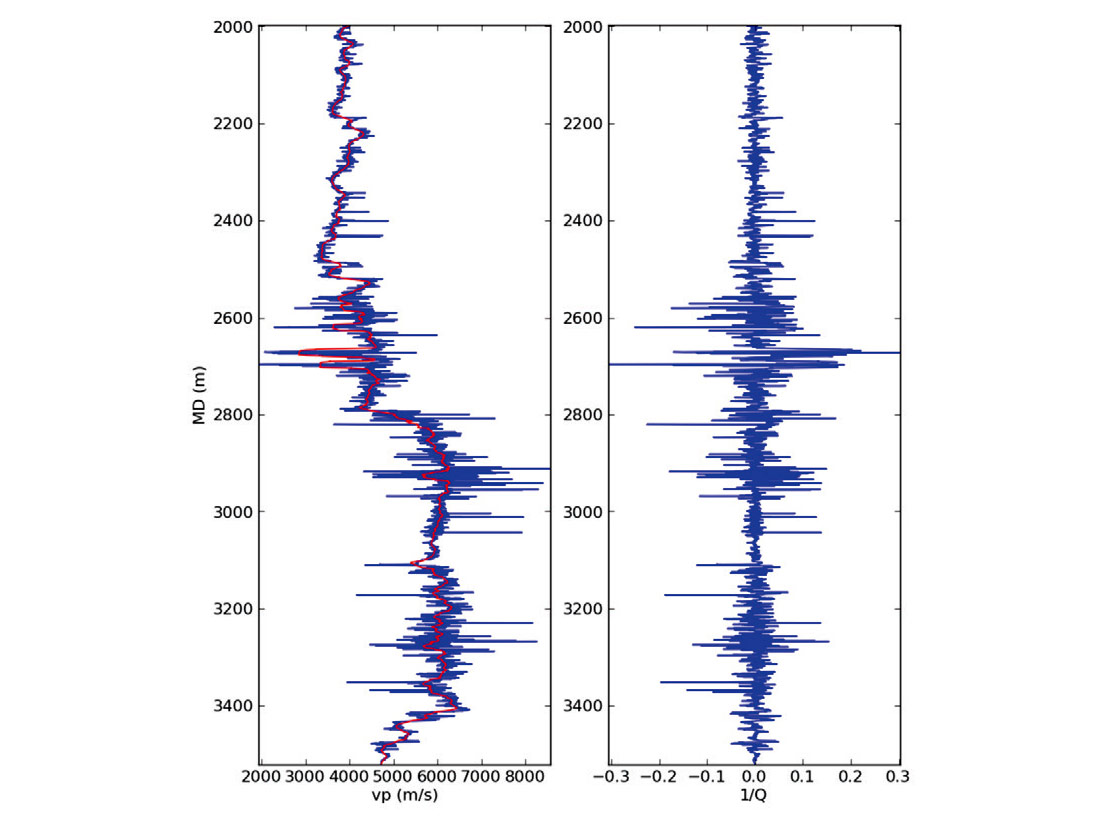
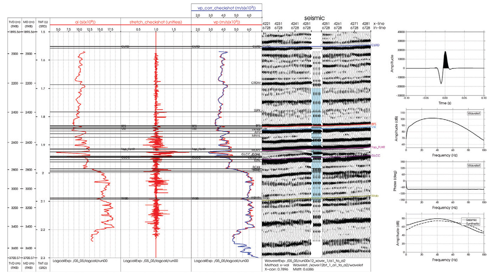
Figure 3 shows the well to seismic tie using a time-depth relationship computed by integrating the Backus averaged slowness. The Backus averaged time-depth relationship was loaded as a pseudo-checkshot to allow for a direct comparison with the original well log derived time-depth relationship. The panels from left to right show the acoustic impedance log, pseudo-checkshot stretch factor, well log velocity and pseudo-checkshot corrected velocity, seismic section with synthetic insert and the wavelet with its corresponding spectral representations. Note the improved tie relative to Figure 1 in the vicinity of the coals where we now have a correlation coefficient of 0.79 in the time window 1.7 s to 2.1 s. The pseudo-checkshot stretch factor represents the ratio, V/V₀ or equivalently, t₀ /t, the traveltime ratio of the seismic to logging frequencies. At the coal intervals, the stretch factor is largest with a value of approximately 1.5, which indicates that the seismic frequencies require a traveltime that is 1.5 times longer than that of the logging frequencies. In terms of the velocities as seen by the logging and seismic frequencies, this implies a difference on the order of thousands of m/s.

Conclusions

The question of the validity of stretching and squeezing and how much is acceptable for well to seismic ties have always been a topic of debate. In this study, we show that in the presence of layer induced long wave elastic attenuation as presented by Liner (2014), stretching and squeezing is mandatory as both positive and negative local Q values are possible. By using a Backus averaged well log to compute the time-depth relationship, an improved well to seismic tie can be achieved. Furthermore, the ratio V/V0 provides an indication of how much stretching and squeezing is acceptable.

The method as presented provides a first pass at adjusting the time-depth relationship to account for dispersion as discussed. However, further adjustments will typically be required as the chosen Backus averaging length only provides the upper bound for the seismic frequencies and does not account for dispersion within the seismic bandwidth. Therefore, this provides an approximation for the effective velocity as seen by the seismic waves. Furthermore, logging errors can still be present that will propagate through the time-depth calculations. Therefore, a manual stretch and squeeze is still required to fine-tune the time-depth relationship but should be guided by the above analysis to obtain a reasonable result.

Acknowledgements

We thank Sitka Exploration and Qeye Labs for supporting this work and WesternGeco for permission to show the data. Andrew Graham, Greg Cameron and Marcello Orizzonte are acknowledged for helpful discussions.