Gaussian-beam polarization-based location methods using S-waves for hydraulic fracturing induced seismicity

Summary

We propose a new method to locate hydraulic fracturing induced seismicity using three-component S-waveforms. The method requires only time intervals around the peak amplitude of the S-wave and does not depend on the arrival-time picking accuracy. The initial-value for the ray tracing is along the direction of wave propagation obtained from the eigenvector associated with the minimum eigenvalue by the Swave polarization analysis. Along the ray paths, the energy is back propagated by weighting a Gaussian-beam factor around the rays. Event locations correspond to the regions with the maximum summed energy in the resultant image. We have successfully applied the method to synthetic data sets with P-wave signal-to-noise ratio down to -2.4dB and to real data from a hydraulic fracture fluid treatment, and examined the sensitivity of the location accuracy to the percentage of S-wave splitting, the signal-to-noise ratio, the receiver network, and robustness to the number of available receivers.

Introduction

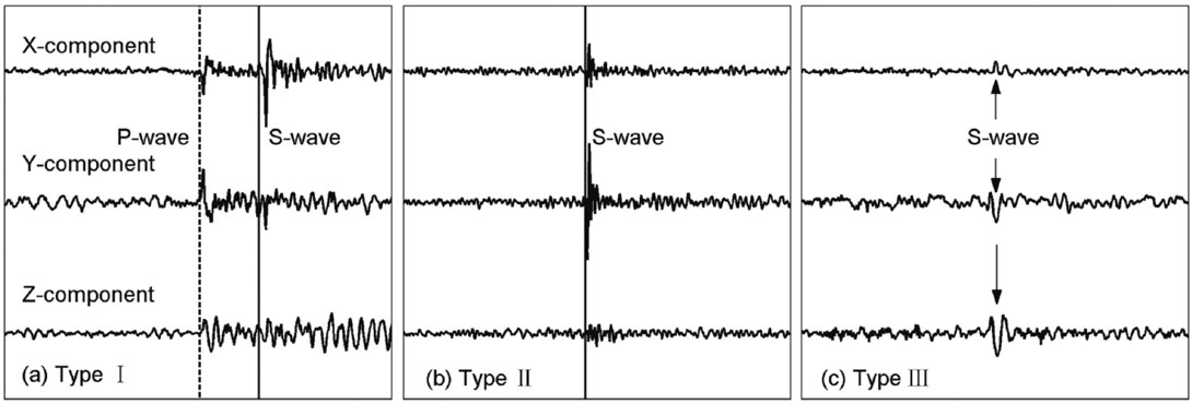
Hydraulic fracturing and microseismic (MS) monitoring are established techniques to improve the production of hydrocarbons from unconventional oil and gas reservoirs [Pearson, 1981; Rutledge and Phillips, 2003; Sharma et al., 2004; Le Calvez et al., 2006; Shapiro et al., 2006], enhance geothermal energy in hot dry rock [Sasaki, 1998; Norio et al., 2008], and facilitate slurry waste re-injection operations [Warpinski et al., 1999]. Accurate 3D locations of induced seismicity provide crucial information about the geometry and propagation of hydraulic fractures [Griffin et al., 2003]. As shown in Figure 1, the triggered MS events can be divided into three types depending on the signal-to-noise ratio (SNR) of the Pand S-waves. MS events often have clear S-waves but their Pwaves are small and difficult to be accurately picked. This is a common situation in hydraulic fracturing due to the high amplitude ratio of S-wave to P-wave generally found in the recorded MS signals, and also an effect of attenuation of the generally higher frequency content of the P-waves.

In order to achieve an accurate location of a MS event induced from hydraulic fracturing with linear receiver arrays, the majority of studies use a combination of P-wave and/or S-wave arrival-times and polarization data [Maxwell and Urbancic, 2001; Fischer et al., 2008]. These location routines strongly depend on the precision of the arrival-time picking which can be done automatically (less accurate) or manually (more accurate, but more time consuming). Also for these methods, Type III events are unusable.

Recently, Rentsch et al. [2007] presented the Gaussian-beam polarization-based method by P-wave with the following benefits: (a) The method only depends on P-wave polarization data; (b) The method can be fully automated; (c) The method can provide locations with a similar accuracy to manual arrival-time picking methods. However, because it only uses P-waves, it can not accurately process Type II events whose P-waves can not be visually identified and Type III events.

The proposed new location method, the Gaussian-beam polarization-based location method by S-wave, hereafter called the S-wave GB method, is based on the method of Rentsch et al. [2007], but focuses on S-waveforms instead of P-waveforms. It can automatically produce 3D locations for all three types of events identified in Figure 1, therefore significantly increasing the ability to discriminate the shape and size of hydraulic fracture zones and significantly reducing the amount of manual (user) processing time required.

Theory of the S-wave GB Method

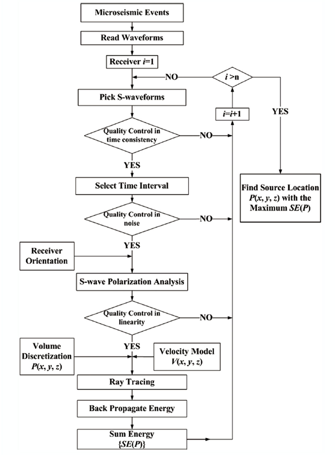
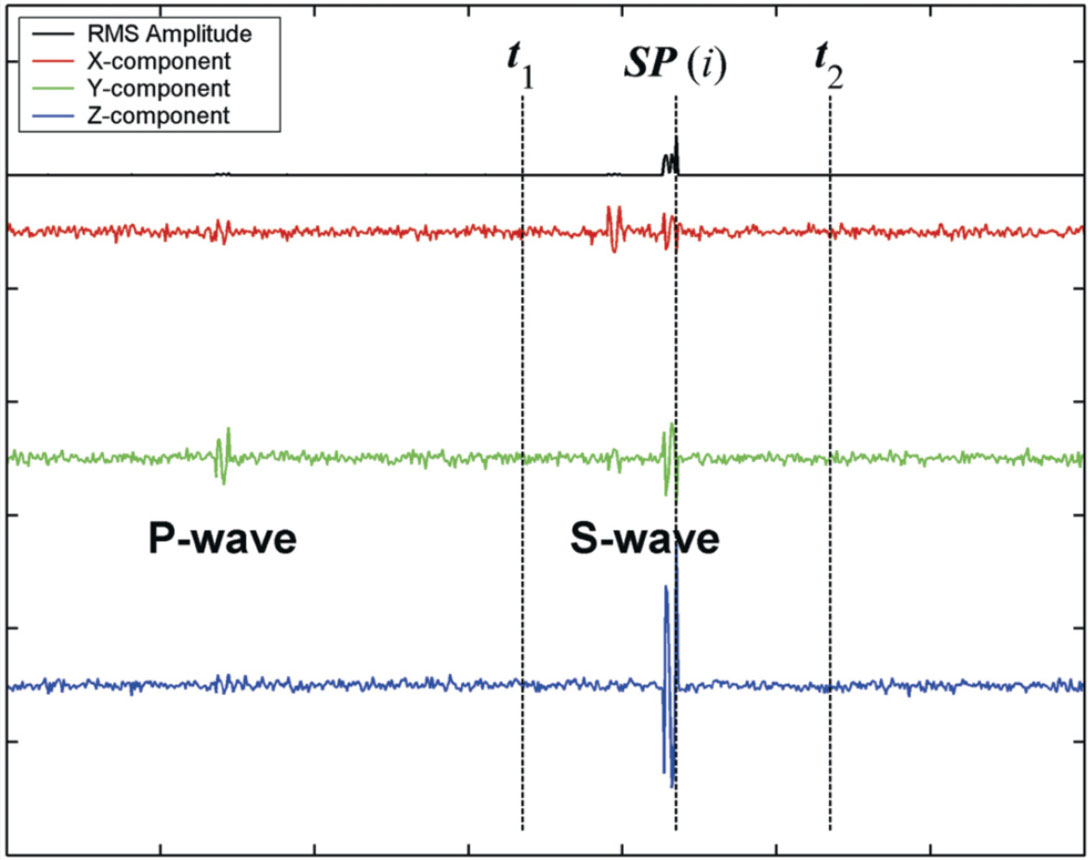
The flow chart of the S-wave GB method is shown in Figure 2. As illustrated in Figure 3, for receiver i (i=1 to n, n is the number of receivers), the S-wave is automatically identified by the sample point with the maximum root-mean-square (RMS) amplitude (denoted by SP(i)) calculated by recorded 3-component waveforms because the S-wave usually has the maximum energy in a hydro-fracturing induced MS event. The time interval is then chosen (from t₁ to t₂ as shown in Figure 3) between several dominant wavelengths before and after SP(i) to include the majority of S-wave energy (both SH-wave and SV-wave). Based on the selected time interval and receiver orientation information, the covariance matrix [Hendrick and Hearn, 1999] is solved to find the eigenvector corresponding to the minimum eigenvalue, which is considered to be the starting direction of the ray in the bi-directional initial-value ray tracing from each receiver.

During the ray tracing in the seismically active volume, the energy within the selected time interval is back propagated to a discretized grid point P(x, y, z) weighted by a Gaussian-beam exponential g(P) defined in equations (1) and (2).

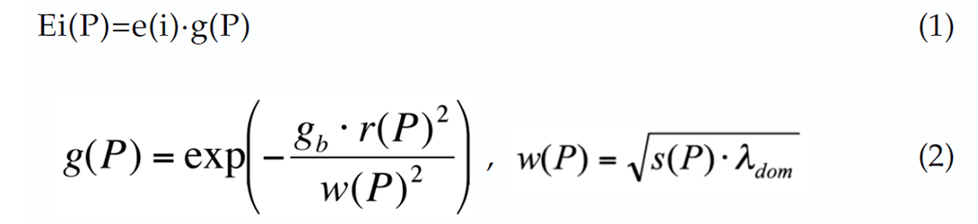
where Ei(P) is the received energy in the grid point P from the receiver i, e(i) is the energy within the selected time interval at the receiver i, r(P) is the perpendicular distance from P to the ray centre, w(P) is the beam width, s(P) is the ray length, λ_dom is the dominant wavelength of the S-wave, and the coefficient g_b is introduced to control energy distribution along the plane perpendicular to the centre ray.

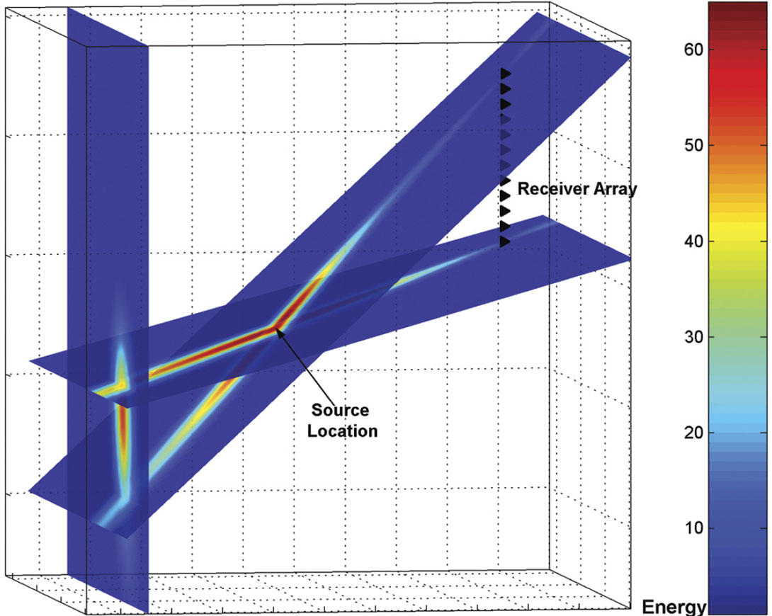
The equations (1) and (2) assume that significant energy values are concentrated within the beam width and decrease rapidly outside the beam width. This is similar to Fresnel zones [Sheriff, 1980] which are directly proportional to the location uncertainty. The effect can be clearly seen in the energy distribution after implementing the S-wave GB method for a synthetic MS event (Figure 4). After calculating the energy for all grid points from all of the available receivers, the summarized energy SE(P) is achieved. The source location is found corresponding to the grid point with the maximum SE as shown in Figure 4.

In addition, the S-wave GB method involves three quality control steps. Firstly, the time consistency is used to exclude receivers with an inconsistent phase identification on SP(i). Secondly, the differences of noise between receivers and within each component are restricted to exclude receivers with high noise level and bad coupling in the three components. Finally, the azimuth reliability and linearity [Hendrick and Hearn, 1999] are implemented to reduce the influence of receivers with an unreliable polarization. As shown in Figure 2, the S-wave GB method is a fully automated location routine once optimal ‘quality control’ values have been determined for any particular data set to be processed.

Results and Discussion

The S-wave GB method was firstly applied to synthetic data sets with a homogeneous and isotropic model. The sensitivity of the method was examined by the following factors: the percentage of S-wave splitting (PSS), the SNR, the receiver network, and the number of available receivers. PSS is defined in Equation (3) with V_sh and V_sv being the velocities for SH- and SV-waves, respectively. For synthetic data, the velocity of SH-wave was fixed to calculate the velocity of SV-wave based on the corresponding PSS. Therefore, the time interval including S-wave energy can be exactly extracted from the synthetic waveform for each receiver. The assumption for synthetic data is reasonable because a clear separation of the body-wave phases can be resulted from the spacing between monitor and treatment wells in the typical hydraulic fracture monitoring situations. Furthermore, since the method is designed for three-component data, the S-waves can also be identified by polarization analysis [Vidale, 1986; Bai and Kennett, 2000]. Even in the worse scenario when background noise is stronger than the S-wave, the weak seismic signal can be detected by the chaotic vibrator method described by Zhao [2006].

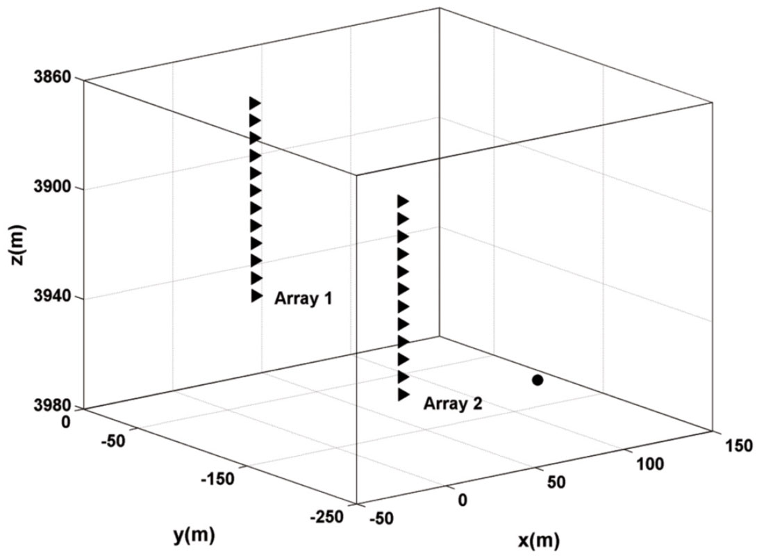
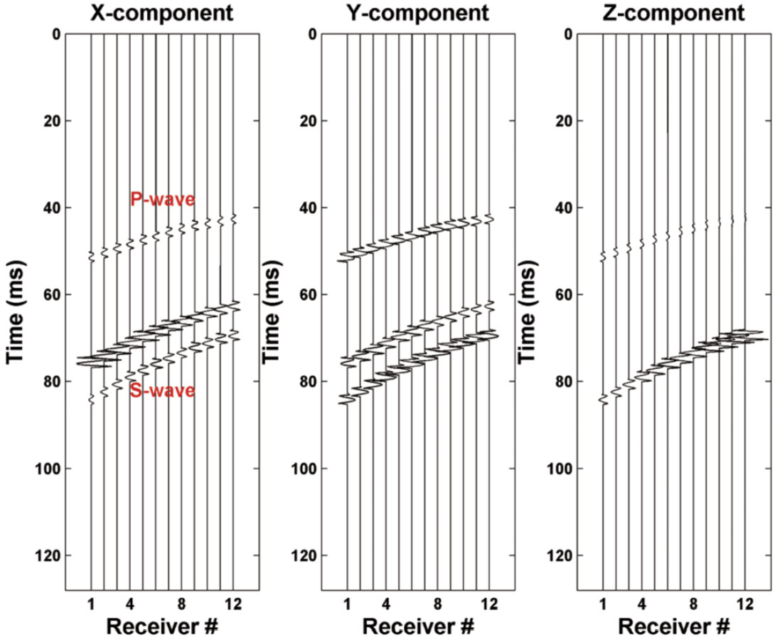
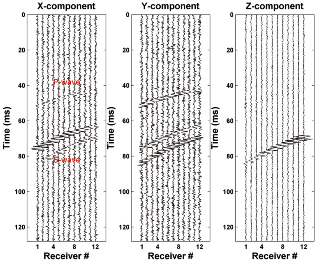
Two types of receiver networks were tested. As shown in Figure 5, the 1D receiver “Array 1” includes 12 receivers whose locations are the actual values from one of the data wells in the fluid treatment on the Bonner sand in the Dowdy Ranch field (east Texas) [Sharma et al., 2004], and the “Array 2” is artificially added to simulate a 2D case comprising the “Array 1” since two monitoring wells were used at the Carthage Cotton Valley gas field (east Texas) [Rutledge and Phillips, 2003] and multiple monitoring wells have become more attractive. For both cases, the source is at x=125m, y=-134m and z=3975m which was the location of the perforation shot, and a double couple source time function was modeled by a Müller-type wavelet [Fuchs and Müller, 1971] with a dominant frequency 500Hz, and velocities 3410m/s for P-wave and 2300m/s for SHwave [Sharma et al., 2004]. The average distance between receivers and the source is about 155m and 177m for the 1D and 2D cases, respectively. In order to compare with the results from the P-wave GB method by Rentsch et al. [2007], all SNR values in this paper were calculated based on the ratio of P-wave to noise. The variable ranges for SNR and PSS are -20dB to 40dB with the increment 1dB and 0.01 to 0.3 with the increment 0.01, respectively. For example, by the 1D receiver array, Figures 6 and 7 show the synthetic seismogram with PSS=0.1 without noise and SNR=5dB, respectively. The S-waves usually have higher amplitudes than the P-waves in the resultant waveforms. Similar seismograms occur for the 2D receiver array but there is a time shift between the Array 1 and the Array 2, as expected.

Consequently, according to the flow chart shown in Figure 2, location errors can be solved for each pair of PSS and SNR. Here the location error was computed by the ratio of the Euclidean length between estimated and actual source locations to the average source-receiver distance, and if the location error is no more than 10% which is similar to the criterion used by Rentsch et al. [2007], the location is regarded as successful. At the same time, we can obtain the angle differences between the actual and estimated ray vectors for all receivers.

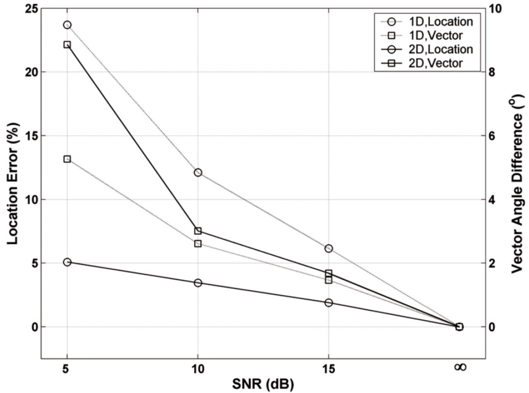
As shown in Figure 8, with no added white noise for Figure 6, the coordinates of the maximum energy are the same as the location of the modeled event. The same result was obtained by the 2D receiver array. With the increase of white noise, the angle difference becomes distinct which results in a larger location error. Noticeably, the higher location accuracy was obtained from a 2D receiver array with a larger vector angle difference as shown in Figure 8. This indicates that if more monitoring wells are available, more accurate locations can be achieved.

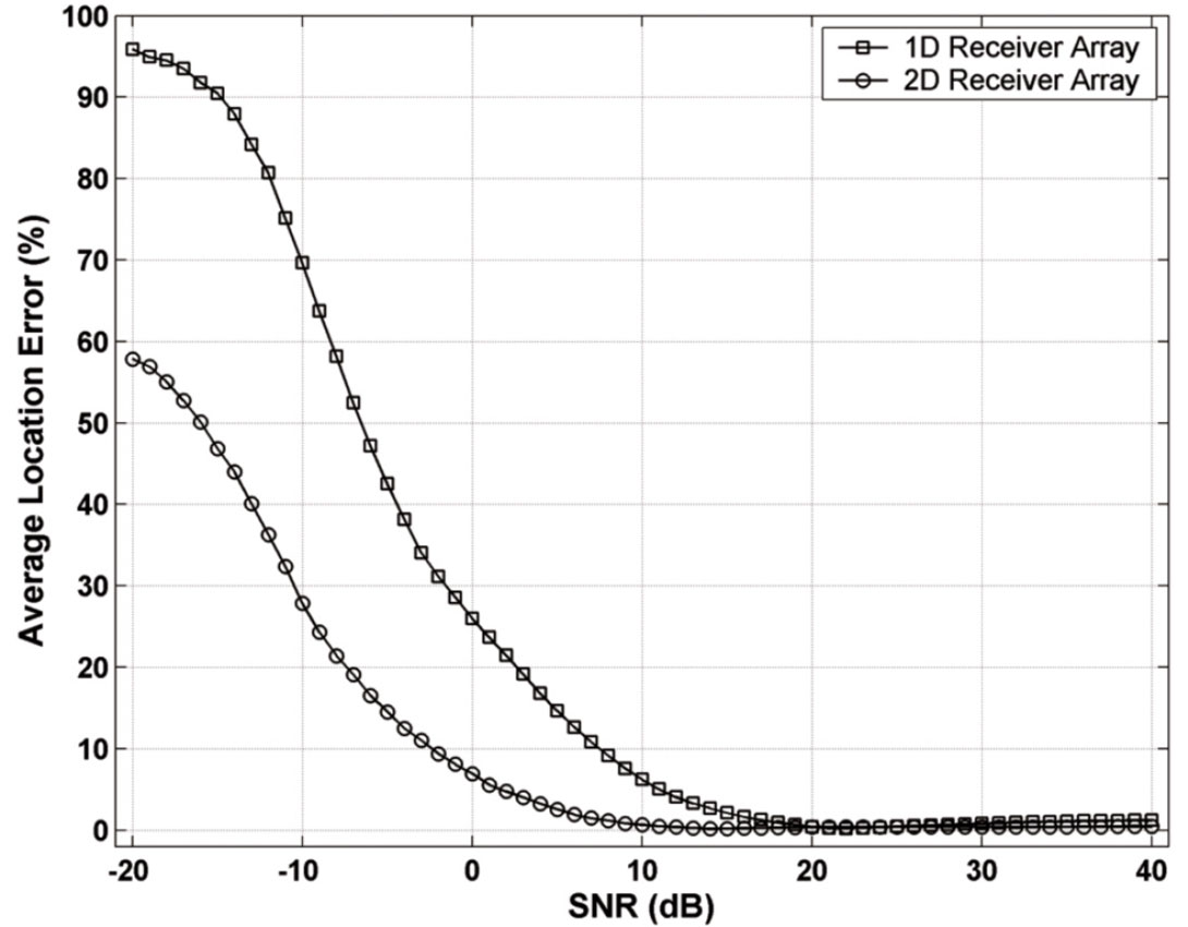
Figures 9 and 10 demonstrate the location errors for each pair of SNR and PSS under the 1D and 2D receiver array, respectively. For each pair of SNR and PSS, over hundred different white noises (104 and 106 tests for 1D and 2D cases, respectively) were tried to optimize the statistic effect of noise on the location accuracy. Based on the results in Figures 9 and 10, the average location errors for both receiver layouts are shown in Figure 11. According to Figures 9, 10, and 11, as white noise is added, the location error starts to increase as expected. The 2D receiver array often achieves more accurate locations than the 1D case because the energy is more focused with 2D receivers. For instance, when PSS=15% close to the average PSS for the Bonner data, the location accuracy under the 2D condition is generally over 5 times higher than that under the 1D case from -10dB to 10dB, which is the area of challenge and interest for seismic signals. Promisingly, the SNR limit with a successful location is down to 7.5dB and -2.4dB for 1D and 2D cases respectively, which have improved the corresponding values from 9.1dB and 6.8dB using the P-wave GB by Rentsch et al. [2007]. In addition, all locations are successful for any PSS when SNR≥9dB and SNR≥0dB for 1D and 2D cases, respectively.

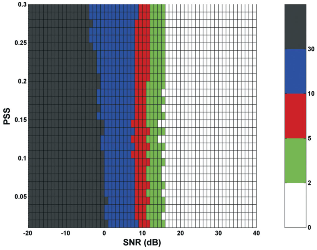
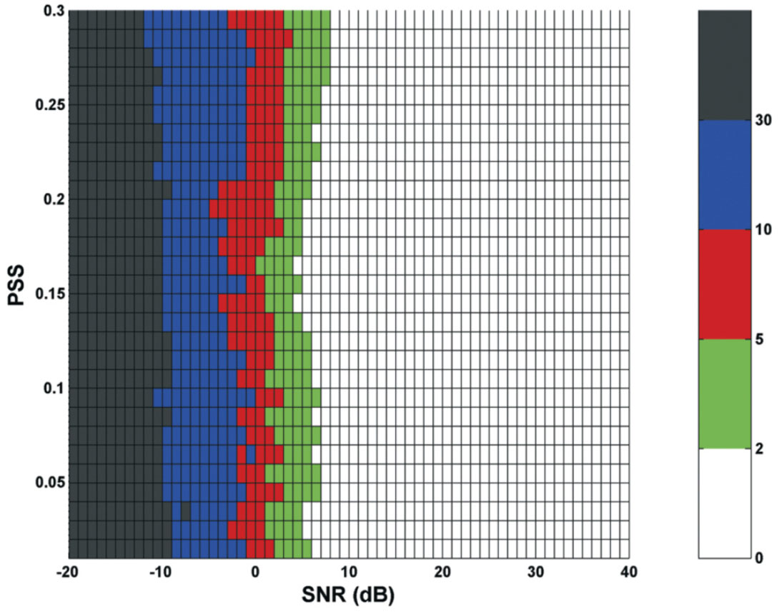
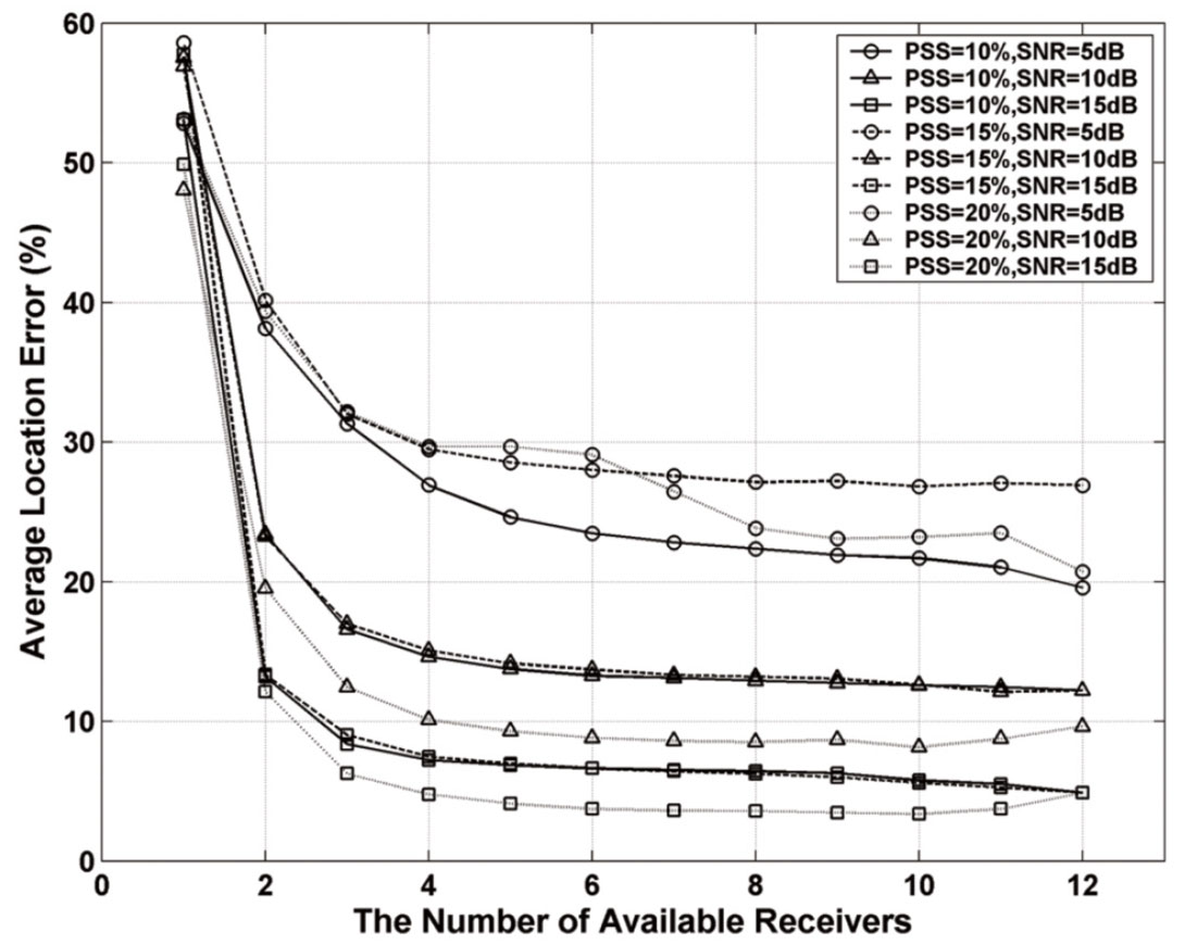
Figure 12 shows the average location errors for all combinations of available receivers under the different PSS (0.1, 0.15 and 0.2) and SNR (5dB, 10dB and 15dB). The average location error shows a general decreasing trend with increasing number of receivers. More specifically, a steep decrease in error is found followed by a general leveling off above a certain number of receivers. Figure 12 also shows that only 4-6 receivers are required to reach a stable solution for the S-wave GB method, indicating the robustness of the method to low numbers of measurements. Moreover, for a certain PSS, the location error starts to increase significantly when white noise is added, while for a particular SNR, varying the PSS has a far smaller influence on the location accuracy.

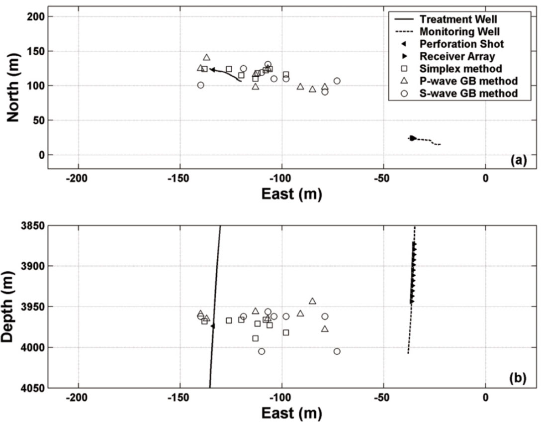
Next, we have applied the S-wave GB method to a subset of the MS events induced from hydraulic fracturing of the Bonner sand, and compared with the results by the P-wave GB method and the event locations by the arrival-time-based method (the Simplex routine [Nelder and Mead, 1965], which is an iterative procedure that searches the error space for a minimum traveltime residuals [Pettitt and Young, 2007]) in Figure 13. The arrival times were manually picked. The average magnitude for all selected MS events is Mw=-0.05. The sample time is 0.25ms and the dominant period is approximately 2ms. A time interval of about 5 dominant wavelengths around P-waves onset were selected, while for S-waves 3 dominant wavelengths before SP(i) and 4 dominant wavelengths after SP(i) were selected. These selected time intervals as well as a simple 1D velocity model consisting of six layers were used for the GB method. Our event locations show a good agreement with corresponding locations calculated by the Simplex method. Moreover, the average location errors are 19% and 21% for the P-wave and S-wave GB methods respectively with an average SNR=7.8dB, which agrees with the synthetic results shown in Figure 11.

Conclusions

A new approach, called the Gaussian-beam polarization-based location method by S-wave, is presented to locate MS events induced by hydraulic fracturing. Characterized by full automation, the approach is less sensitive to picking precision compared to more traditional location techniques. The polarization information is found using only S-waves, and the event location is deduced from the maximum stacked energy in the resulting energy distribution. Our tests on synthetic data sets have shown that the location errors are mainly affected by the signal-to-noise ratio and less affected by S-wave splitting. Additionally, only 4-6 receivers can satisfy a robust stable solution, with additional sensors having only a small increase in location accuracy. Promisingly, the method can successfully locate (defined as a location within 10% of its true location) synthetic events with SNR down to -2.4dB if a 2D receiver network was deployed similar to the Carthage Cotton Valley data set. For the MS events from the fluid stimulation on Bonner sand, all of the locations obtained by the S-wave GB method were in reasonable agreement with the results obtained by the arrival-time based location routine. The average SNR of the induced MS events and calculated location error are in good agreement with results from the synthetic tests, suggesting that the SNR of MS events is directly proportional to location accuracy.

The S-wave GB method has the potential to locate all three of the types of hydraulically induced MS events defined in this study. However, in order to retrieve more hydro-fracturing induced MS events, further developments should examine the polarisation uncertainty of S-wave, waveform phase identification at a low SNR, as well as the uncertainties in the S-wave velocities.

Acknowledgements

We thank Applied Seismology Consultants Ltd. and the Halliburton Company for providing the hydraulic fracturing datasets.