A Convenient Truth: Radial Trace Filtering—Simple and Effective

Introduction

Seismic processing sometimes has something of a “mystique” associated with it, that compels us to use only the most theoretically correct or sophisticated algorithms to accomplish specific tasks on our data sets. Because of this, we sometimes overlook or ignore methods which are not as intellectually satisfying, but which, nevertheless, can be very effective in spite of their simplicity. One tool which might well fall into this category is the Radial Trace (RT) Transform, introduced to the seismic world by Claerbout et al (1975, 1983), and Taner et al (1980) many years ago. Because it is a simple point-to-point mapping, like NMO correction, but unlike the better known integral transforms like the 2D Fourier Transform, or the Radon Transform, its usefulness has been under-appreciated by seismic processors...in fact, many seismic processing toolkits have no algorithm for performing the transform and its inverse. The intent of this article is to re-introduce the Radial Trace Transform to seismic processors and to illustrate one of its more useful applications: coherent noise attenuation (Henley, 2000, 2003).

The RT Transform: What is it?

The Radial Trace Transform can be envisioned as overlaying a seismic trace gather (a matrix in source-receiver offset, X, and two-way travel time, T) with a fan of constant-velocity trajectories radiating from a common origin, then extracting samples along each of the linear trajectories from the underlying seismic traces, interpolating when necessary. The samples along each radial trajectory become a single trace in the new (RT) domain (a matrix in apparent velocity, V, and two-way travel time, T). Just as the source-receiver offset X uniquely identifies each trace (column) in the original seismic trace gather, each trace in the RT transform is identified by the apparent velocity, V, of the radial trajectory along which its samples were collected in the XT domain. Figures 1 and 2 illustrate this process. Because of the non-uniformity of its sampling trajectories relative to the XT domain (diverging from a common origin), the RT transform must over-sample the original XT domain, in order to capture details of the original trace gather around its perimeter without aliasing. Hence, interpolation is an integral part of the radial transform algorithm. Many interpolation schemes can be used in the RT transform, but the most common implementation is a one-dimensional interpolation along the constant-T rows of the original XT matrix, often involving only the two traces nearest the desired interpolated sample. Whereas NMO correction is interpolation of each column of the XT matrix to form a new XT₀ matrix, the RT transform is interpolation of each row of the XT matrix to form a VT matrix (apparent velocity and travel time).

Why the RT Transform Works for Coherent Noise

The basic principal used to attenuate coherent noise is to find a domain in which signal and noise are well separated within the domain coordinates, so that the noise can be suppressed in that domain, without affecting signal, or, alternatively, estimated and then subtracted in the original domain. This is the basis for multi-channel filtering techniques such as f-k filtering, or multiple attenuation in the Tau-P domain. An indication as to how well a particular domain will work for coherent noise attenuation is how ‘compact’ the representation of the noise is in the new domain; that is, does the region spanned by the noise in the XT domain ‘collapse’ to a much smaller region in the new domain, and does the entanglement of the noise and desired signal significantly decrease? Does the pattern of ‘trajectories’, or ‘components’ which carry samples from the XT domain to the new domain (either by direct mapping, or by summation) closely fit the pattern of either the signal or the coherent noise in the XT domain? Pattern matching is the basis for much of the design criteria for f-k filters, and, more intuitively, for the linear, hyperbolic, and parabolic forms of the Radon Transform. In the case of the RT transform, it is also intuitively obvious that its pattern can be a natural fit for almost any coherent noise, especially that generated by the seismic source.

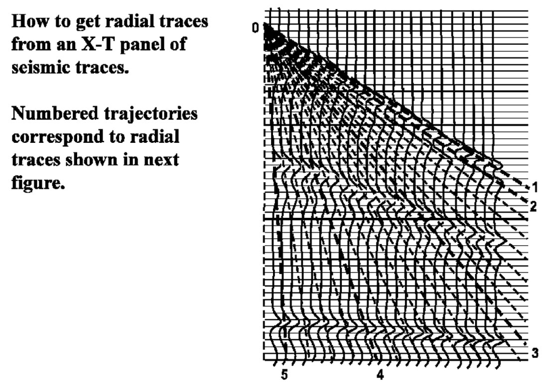
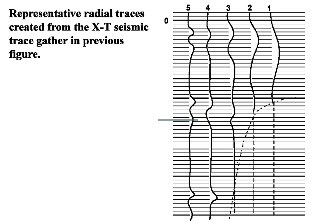
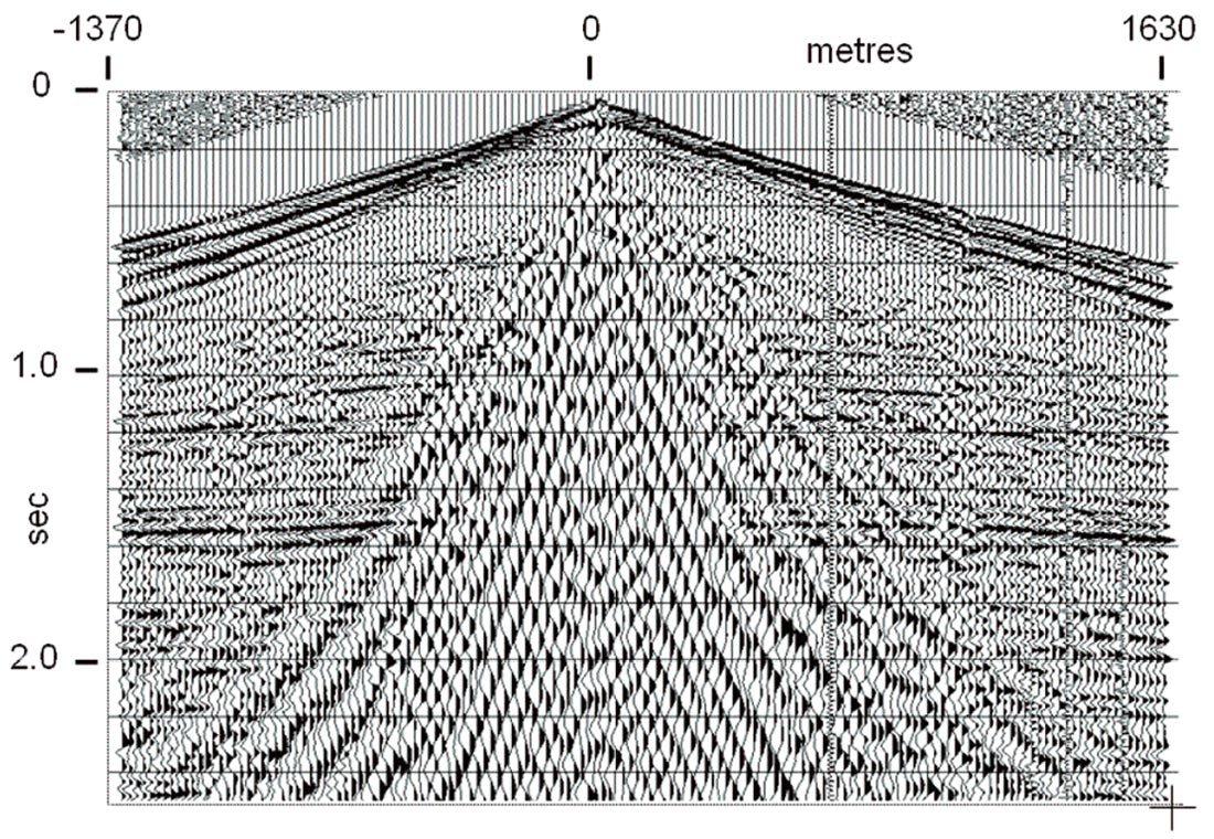
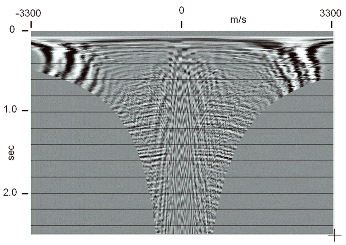
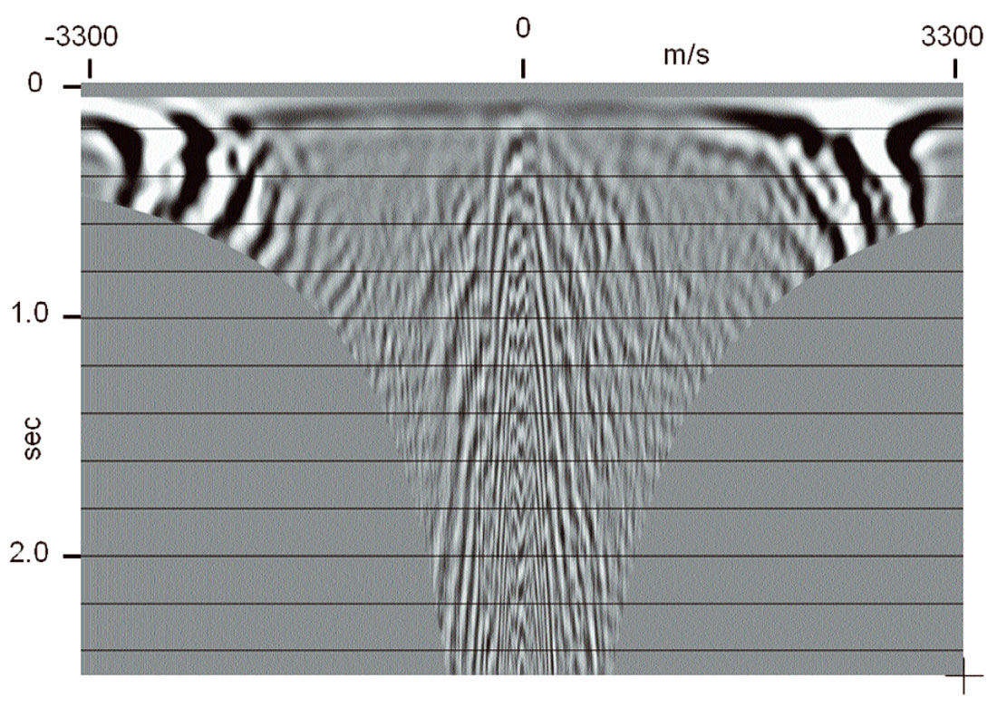
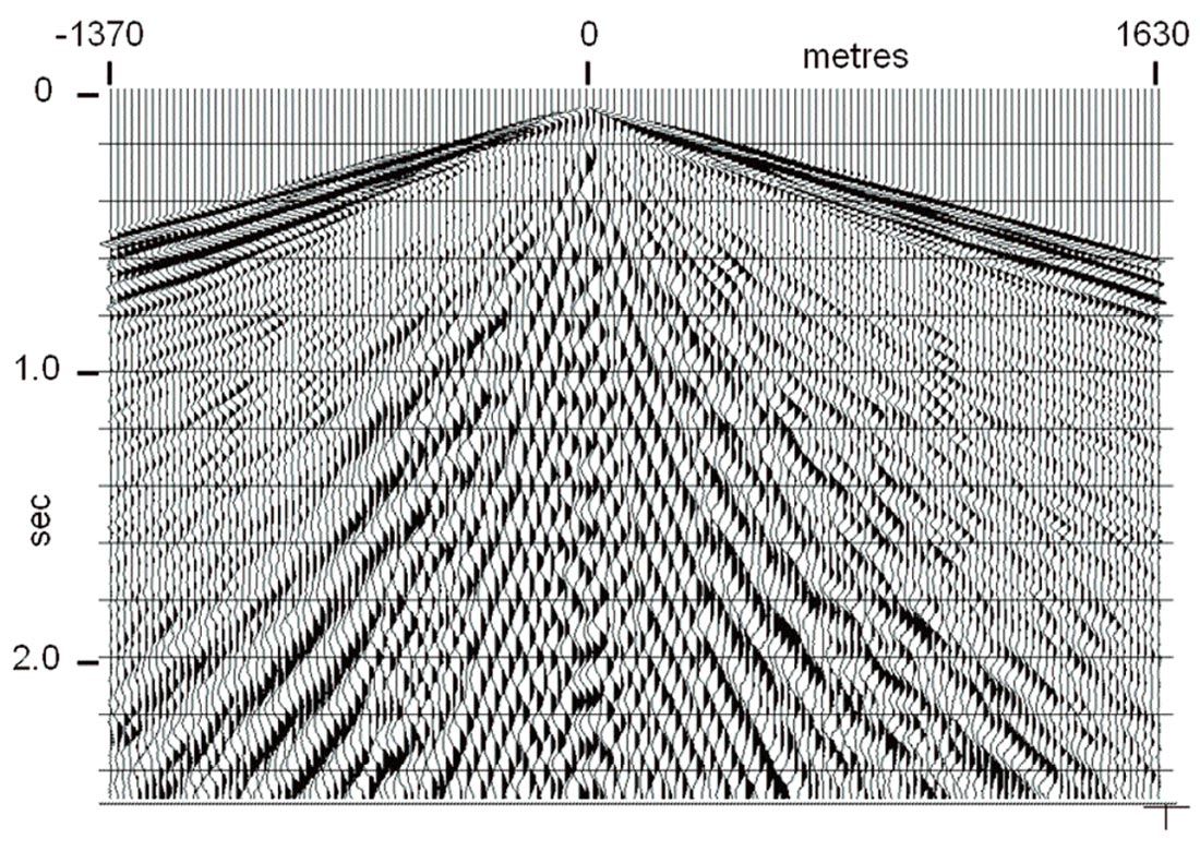
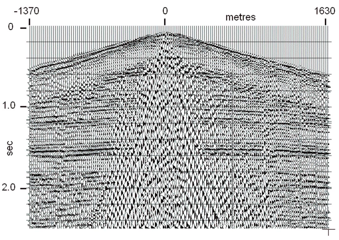
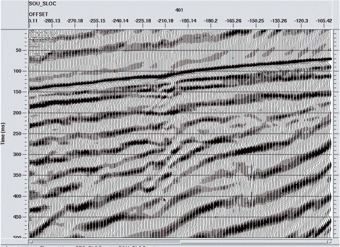
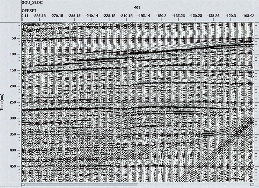
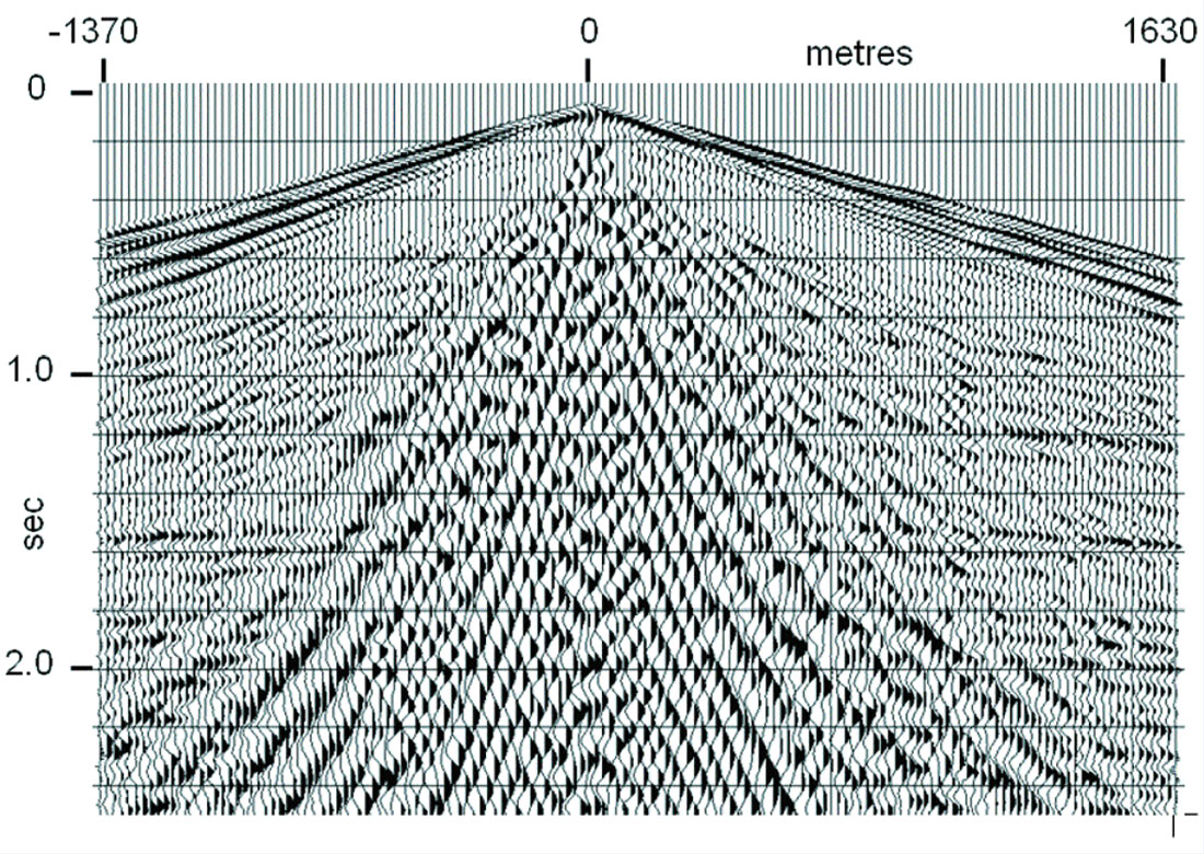
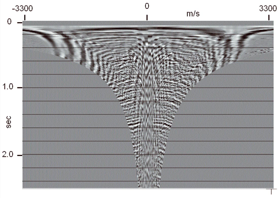
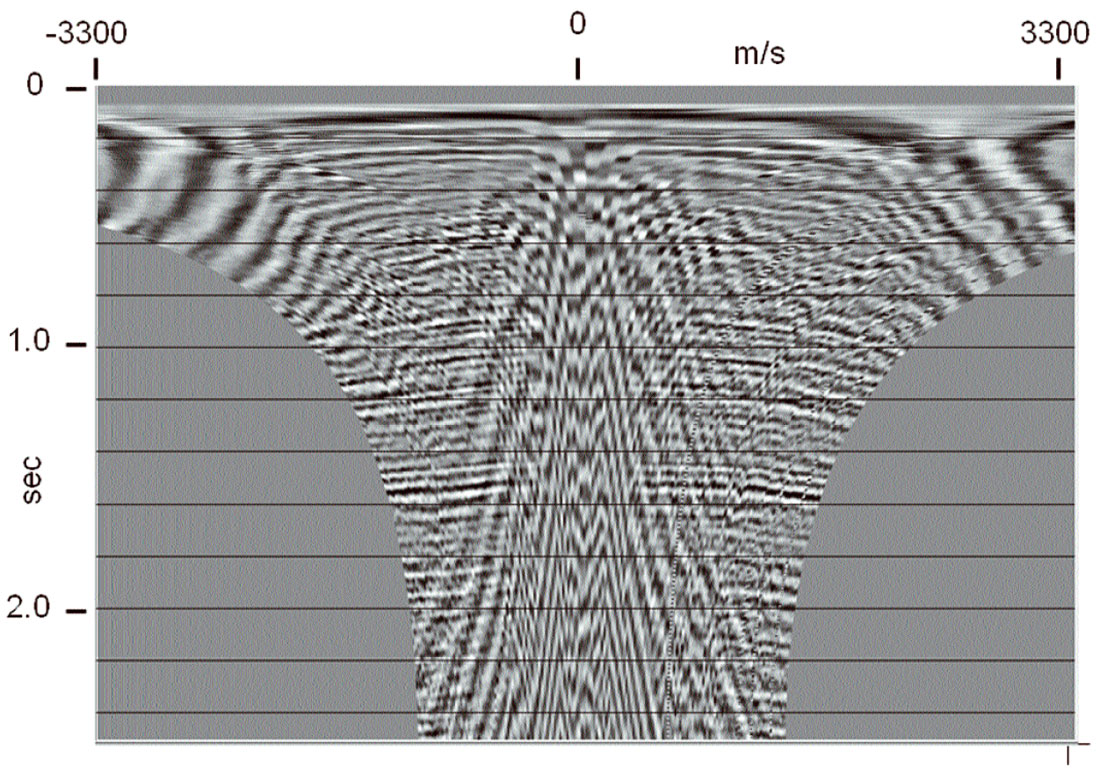
Because the trajectory pattern of the RT transform (see Figure 1) is a fan of straight lines radiating from a common origin, it matches the pattern of much of the source-generated coherent noise radiating away from the source point on a typical source gather. By choosing an appropriate range of velocities and placing the origin of the RT transform at the apparent source position of a source gather, the transform will efficiently capture source-generated noises of any velocity within the selected range. Furthermore, because the trajectories are very nearly parallel to their constant-phase wavefronts, the noise events will be very low in frequency (ideally, zero) in the RT domain. Hence, a specific linear coherent noise event passing through the RT origin will be isolated into a relatively small number of traces in the RT domain and will manifest only low frequencies. Figure 3 shows a typical shot gather with strong high velocity direct arrivals and shallow refractions, as well as lower velocity g round roll. Note, also, the three isolated noise traces in the right hand part of the gather, as well as some small statics jitter evident in the reflections. Figure 4 shows an RT transform of this gather; and it can be seen that the linear noise has been isolated into relatively small groups of traces, and, more importantly, that it is much lower in frequency. Removing this noise is as simple as a low pass filter in the RT domain to remove reflections, followed by RT inversion and subtraction of the noise estimate from the original gather. Figure 5 shows the low-pass of the RT transform in Figure 4, and Figure 6 is the inverse RT transform; the noise estimate to be subtracted from the original shot gather. Notice that no reflection energy leaks into this noise estimate. Figure 7 shows the subtraction result, a shot gather with greatly reduced noise. Furthermore, there is virtually no smearing of events, as often occurs with f-k filtering, and no inversion artefacts, as often occurs with Tau-P methods. The three noise traces in the right hand part of the gather in Figure 3 have survived the filtering process without lateral smearing, as seen in Figure 7, as have the statics.

The advantage of RT filtering methods is that a filter can easily and intuitively be fitted to the actual noise present on a shot gather, just by matching the ‘pattern’ of the noise with that of the RT transform. For noise obviously originating at the source, the RT fan filter, as described above, is quite effective. For repeated sub-parallel noise events with a nearly constant velocity (for which fk filtering is especially well suited) we can pretend that these events have a ‘virtual source’ at some large offset distance from the actual source, and can construct a ‘thin fan’ radial transform whose trajectories have the correct velocity to capture the parallel noise events. In the ‘thin fan’ mode, an RT filter pass is a very effective dip reject filter, which does not smear traces.

Recent Examples

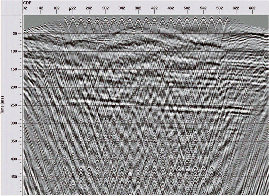
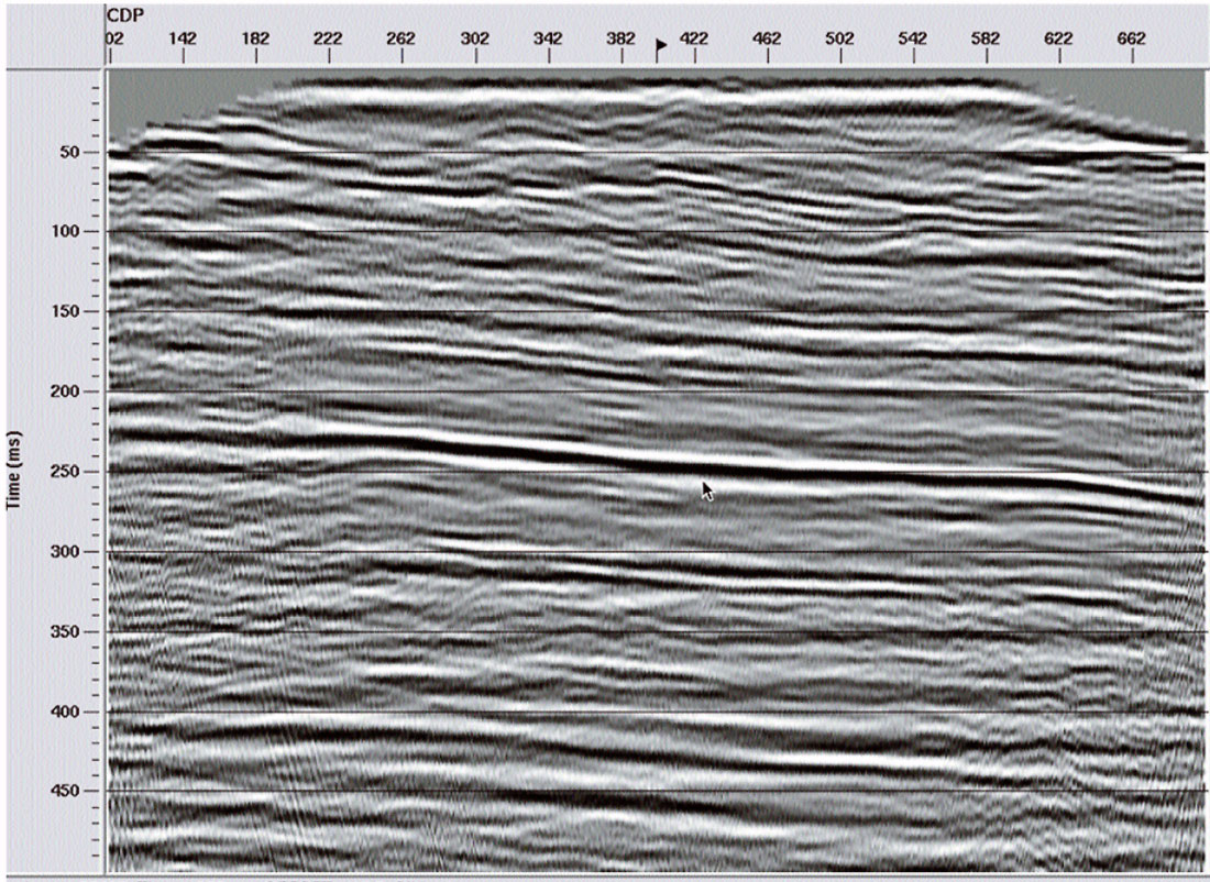
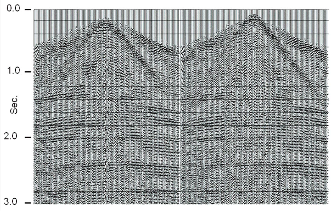
Since we usually use the RT filter technique in the ‘estimate and subtract’ mode, it can be used several times in succession on the same trace gather to remove specific noises one at a time. We usually first apply a fan filter with origin at the source point. After removal of this first layer of noise, we can often see specific linear events or parallel series of events whose velocity can be determined and used to design a thin fan or ‘dip’ filter to remove them. We find that even shot gathers whose reflections are literally ‘buried’ in noise can be filtered remarkably well using this step-wise technique. Figure 8 shows a high-resolution shot gather from an experimental line with 2.5 m receiver spacing. Nothing is visible on this raw record except coherent noise of various kinds. A single pass of an RT fan filter results in the gather shown in Figure 9, while several more RT filter passes, aimed at specific patterns of dipping noise result in the gather in Figure 10. Deconvolving this gather, to recover lost signal bandwidth, results in Figure 11. Though the events in Figure 11 look flat, due to the aspect ratio of the display, they do, in fact, exhibit seismically realistic NMO. Filtering and deconvolving all the shots on this line, then correcting the NMO, we obtain the CDP stack of this line in Figure 12. While the events on this section appear flat, there is, in fact, a slight structural slope of a few ms/km.

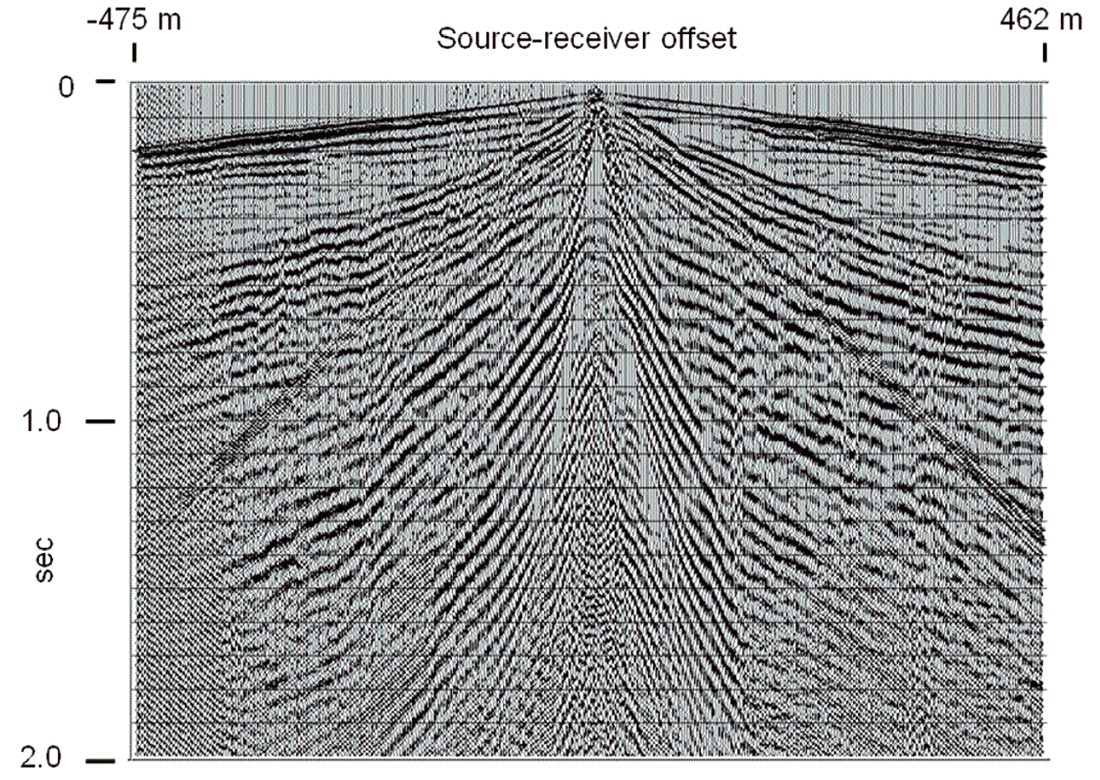
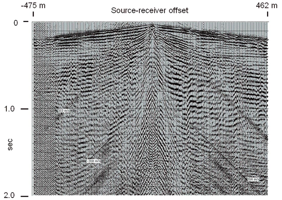
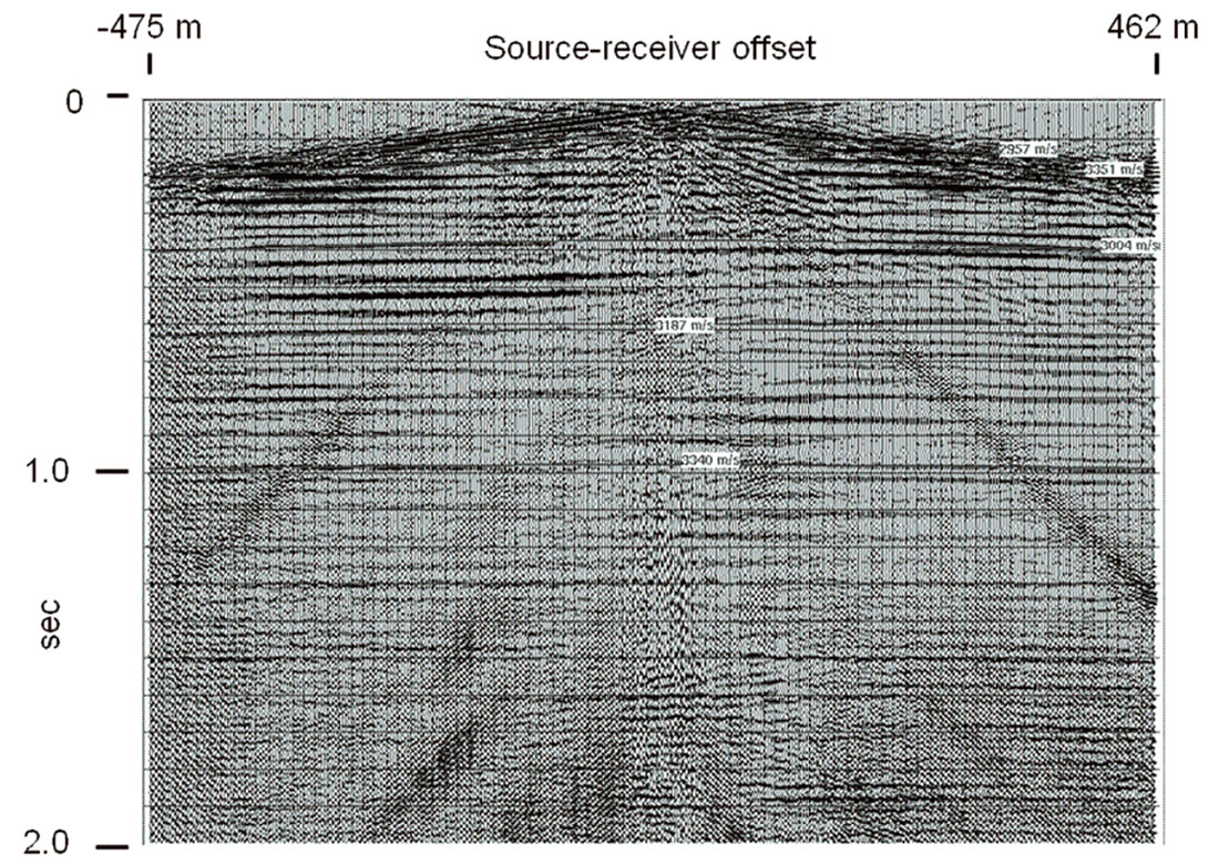
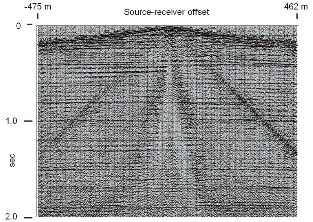
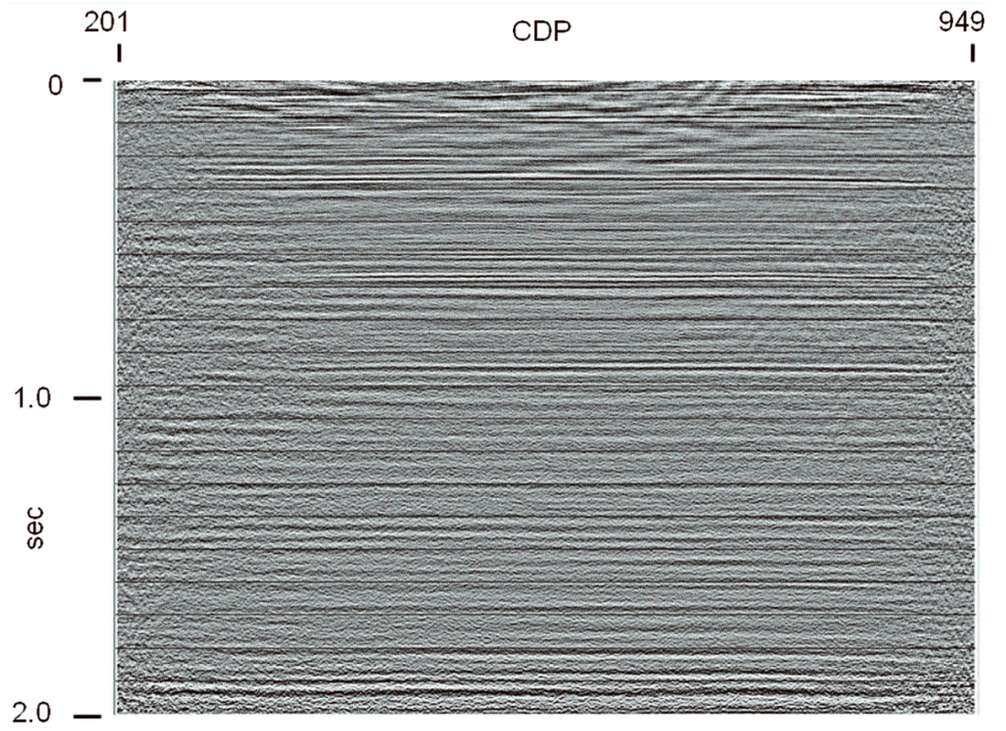
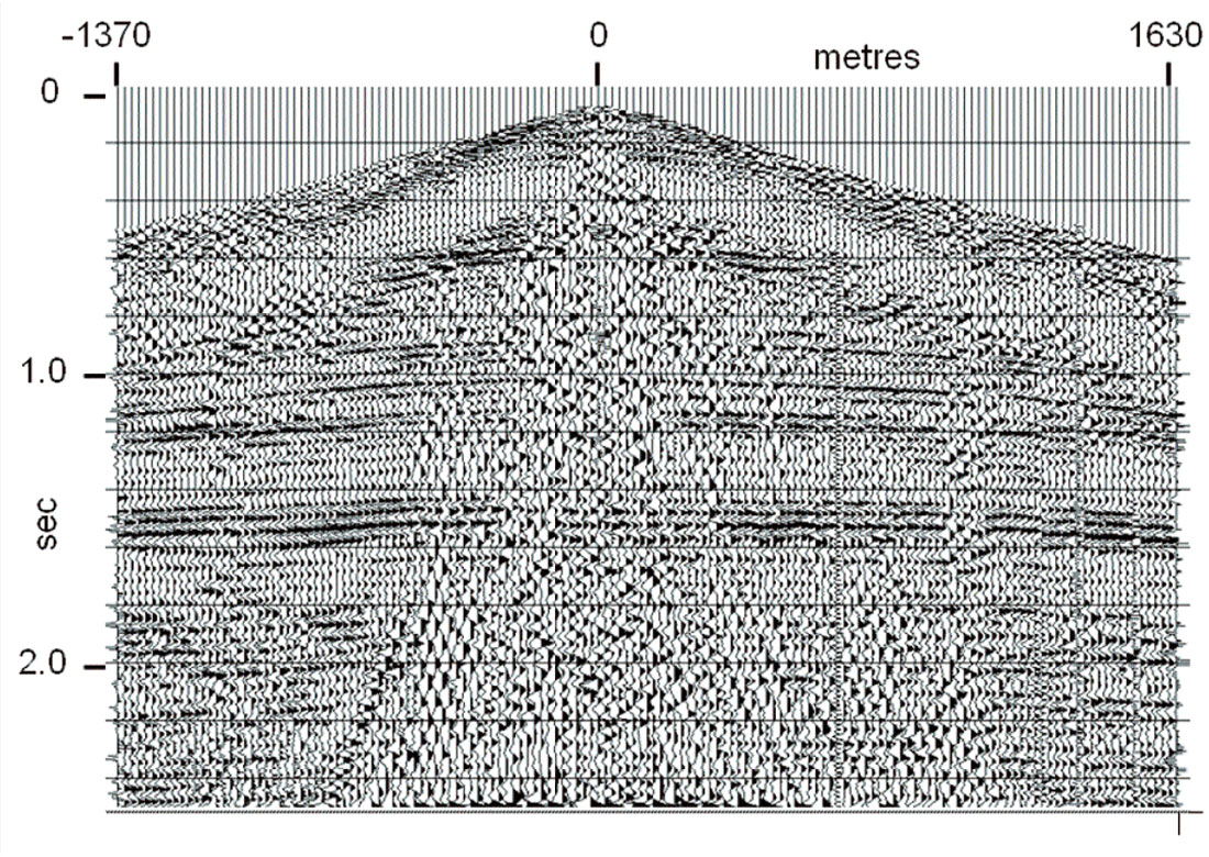
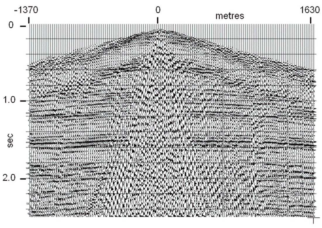
Since we’re always uneasy with conspicuously flat or nearly flat events after application of multiple filter passes, even with a non-smearing technique like RT filtering, we show a second, more recent high resolution example in which there is geological structure. Figure 13 displays a shot gather from a recent field experiment where the receiver spacing was further reduced to 1 m. Similarly to Figure 8, only noise is visible on this raw gather. A cascade of RT filters, followed by Gabor deconvolution (Margrave, et al, 2002) results in the gather in Figure 14, on which many reflections, with discernible NMO, may be seen, even immediately beneath the remnant of the greatly attenuated direct arrival. A brute stack of the raw gathers on this experimental line yields Figure 15, in which only a few prominent reflections can be seen beneath the coherent noise. The filtered and deconvolved gathers, however, lead to the section in Figure 16, with its greatly increased S/N, bandwidth, and detail. Since these events exhibit geological structure, we know that they are real, and not filter artefacts of some kind.

Other Tricks

One of the attractions of attenuating coherent noise in the RT domain is the flexibility of the approach, and the variety of techniques which may be applied in the radial trace domain to separate signal and noise. We have described above only one of many such techniques, in this case using the bandwidth separation of signal and linear noise induced by the radial trace transform to estimate and then subtract the noise. Alow-pass filter is only one of many 1D methods which can be used to isolate coherent noise in the RT domain (running mean, running median, prediction error filter, etc.), but it remains one of the most effective.

Because a radial trace transform is a 2D ensemble, just like its original XT panel, it can also be fruitfully filtered with a 2D filter, especially since the angular separation of reflections from coherent noise is usually greater in the RT domain (coherent noise is mostly vertically oriented, parallel to the T axis). Figure 17 shows a noise estimate obtained by applying an f-k filter to the RT transform shown in Figure 4, and Figure 18 shows the result of subtracting this estimate from the original shot gather of Figure 3. Close inspection of Figure 17 shows that some reflection energy has leaked into this particular noise estimate; but with more careful f-k filter design, this leakage can be reduced. Figure 18 shows that multi-channel noise separation in the RT domain may possibly be more effective than single channel methods, like bandpass filtering, but that filters can be more difficult to design.

Our preferred RT domain noise attenuation method is an estimate- and-subtract scheme, and there will often be some residual noise after the subtraction. As with other such methods, radial trace filtering may be iterated, applying more than one pass of the same filter to a given shot gather. Figure 6 shows the first noise estimate for the shot gather in Figure 3, but Figure 19 shows the second estimate (after subtraction of the noise in Figure 6), and Figure 20 shows the result of subtracting this new estimate from the filtered shot in Figure 7, a significant improvement over Figure 7. The noise estimate in Figure 19 has been scaled for display—its actual amplitude is much less than shown here. Usually, only the first and possibly the second iterations provide worthwhile improvement.

While the estimate-and-subtract technique is the simplest and most obvious coherent noise attenuation method using the RT domain, other methods can easily be devised for separating specific coherent noises in this domain. Figure 21 shows shot gathers on which the air blast is so strong that the display AGC suppresses the trace energy immediately preceding the air blast arrivals. In an RT transform of one of these gathers, however, the strong air blast arrival will be captured by the few radial traces which align with the noise, which will then have much larger amplitudes than neighbouring radial traces. Simply equalizing trace amplitudes in the RT domain, with no further processing, will dramatically attenuate this noise, as demonstrated in Figure 22. This simple trick is not consistent with AVO processing, but you can’t analyze AVO on reflections you can’t see!

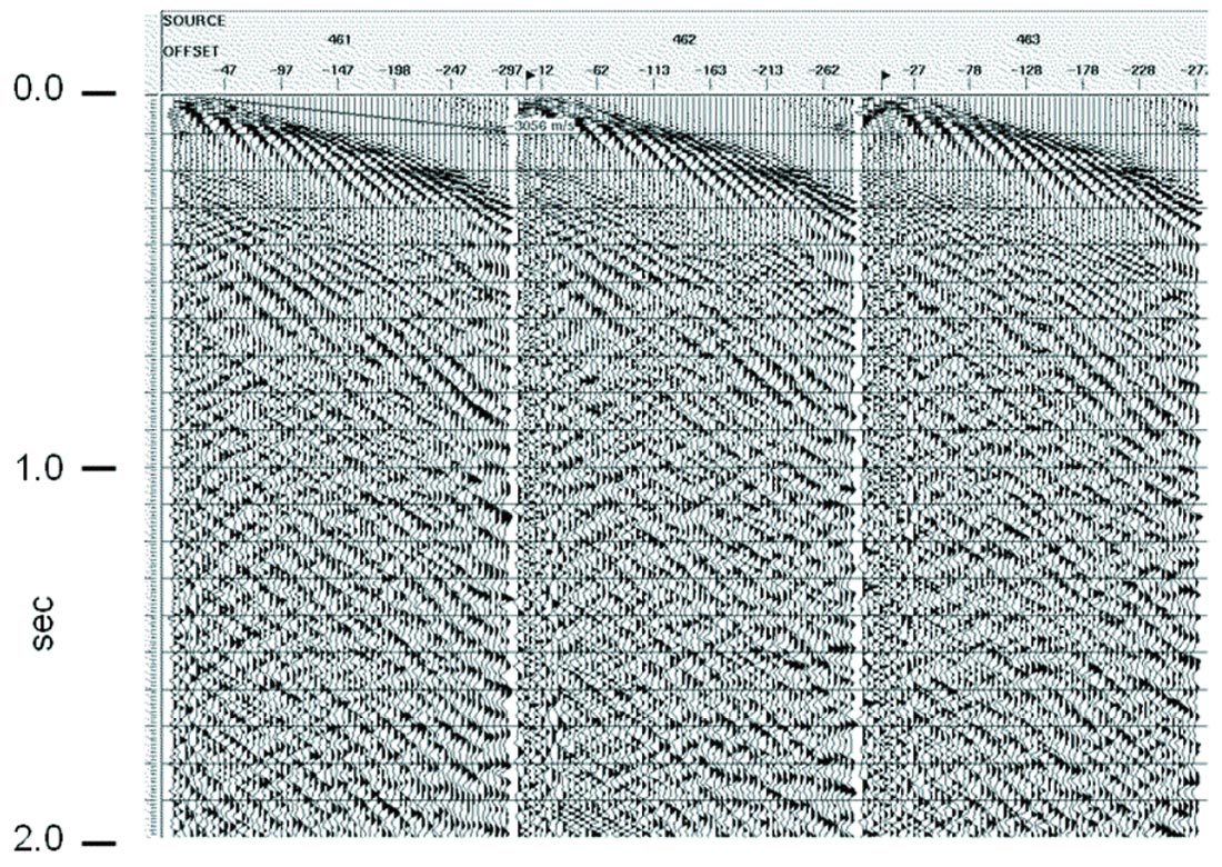
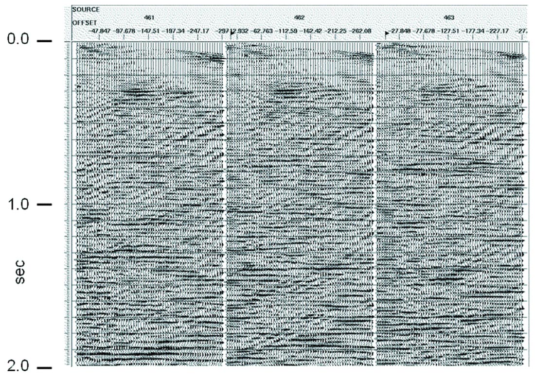
The radial trace domain is also ideal for dealing with coherent noise exhibiting large dispersion, a type of noise where f-k methods are rarely effective. A good example is the ice flexural wave observed when acquiring seismic data on floating ice in the Arctic (Henley, 2006). Figure 23 shows three shot gathers where uniform-thickness ice covering a river channel supports flexural waves which reflect back and forth between the river banks. No reflections are visible on these records, since the flexural wave amplitude is as much as 70 dB above reflection amplitudes. Because of the large dispersion, where each frequency in the wave travels at a different apparent velocity, each trace in an RT transform of one of these gathers captures a single frequency (and its harmonics) of the coherent noise. Hence, the spectrum of each radial trace contains very narrow amplitude spikes, which can be detected and eliminated via a non-linear editing process called ‘spectral clipping’. Spectral clipping in the RT domain, followed by inversion of the RT traces back to the XT domain results in Figure 24, in which it can be seen that there are reflection events beneath the residual noise. This residual can, in turn, be further attenuated by the application of further radial filter passes in the ‘dip filter’ mode.

The standard radial trace transform allows the user to place the radial trace origin, but usually assumes constant velocity linear trajectories for mapping samples from the XT domain. The velocity of any particular radial trace can easily be made a function of travel time, however, so that the trajectories can be made more conformable to the coherent noises they attempt to capture. Figures 25 and 26 show examples of RT transforms in which the velocities of the radial traces are linearly increasing with time or decreasing with time, respectively. It is easy to see the effect of these changes on the coherent noise and its localization and apparent frequency in the RT domain. Such distortions of the original mapping can sometimes be used to improve the effectiveness of an RT filter pass.

3d Issues

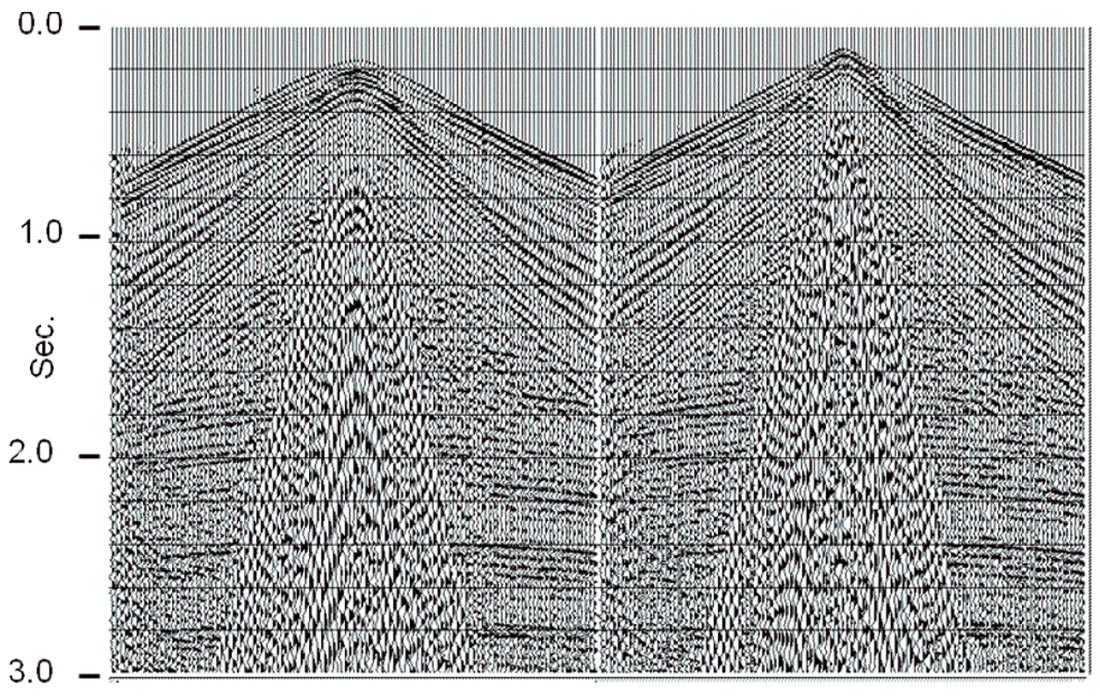
Perhaps surprisingly, radial trace filtering, which is essentially a 2D process, can easily be applied to 3D data. The simple trick is to recognize that receiver line gathers, as conventionally acquired in the field, provide the best-sampled representation of all surface waves and are thus the ideal ensembles for filtering the noise. Each receiver line gather can be filtered as if it were a split-spread 2D shot gather. The only requirement is that the source-receiver offsets, which are posted as absolute distances on most 3D survey traces, be modified to ‘signed offsets’ as in a 2D survey. Since the RT transform is an interpolation process, the fact that offsets are non-linear for receiver line gathers is of no concern, as it would be for f-k filtering or most other multichannel filtering operations. Figure 27 shows a pair of receiver line gathers for a 3D survey, while Figure 28 shows the result of applying RT filtering. Since surface waves are essentially 2D waves, in contrast to the 3D body waves representative of the reflections, it makes perfect sense that we can successfully attenuate them with 2D filters.

Final Comments

Separation and attenuation of coherent noise in the radial trace domain is not a very ‘elegant’ method based on deep theory, but it is a simple and intuitive one. In some cases, it can be more effective than some of the more conventional noise attenuation methods. It is best practiced as an ‘estimate and subtract’ technique, and as such demonstrates no tendency to laterally smear trace amplitudes or statics. Because its sampling trajectories have both apparent velocity and a common origin, the RT transform can, by careful placement of its origin, effectively attenuate linear noise almost parallel to the long offset limbs of reflections, a task beyond the capability of f-k filtering. Likewise, some very dispersive noises, like the ice flexural wave and some examples of ground roll are very difficult to handle in the f-k domain, but yield more readily in the RT domain.