Value of Integrated Geophysics

Many Correlation Coefficients, Null Hypotheses, and High Value

The language of the modern interpreter has a diverse vocabulary. Our action words take the form of recommendations and advice. The geophysicists’ theme, or message, must be one of value. That message is best carried fundamentally by sound principles in physics and geology, and whenever possible gives its voice in a quantitative fashion. However diverse the conversation, the modern interpreter’s sentence structure follows the scientific method. The syntax and the adjectives of this discourse are often statistical. But the sound and fury of statistics are not always as well known as is required for the increasingly quantitative and value oriented song we must sing.

It is well worth discussing some of the statistical tools with which we must measure our results. Most geophysicists learn statistics on an as needed basis; only a few learn or have time to learn of statistics in depth. Some of the really useful articles on statistics assume too much background knowledge. We discuss a few of the basic tools of statistics that are commonly used by geophysicists. Our discussion takes simple form, and points out some sources which may be useful in a more thorough study of the topics we look at. In particular we speak about linear regression and the correlation coefficient. We also discuss statistical significance and the null hypothesis, step-wise multi-variate regression and cross-validation.

This column cannot replace reading a statistics textbook, taking statistics classes, or reading up on the pertinent literature elsewhere. It can, however, open the door to some of these opportunities. Think of this as a gateway to other gateways, or as a sentence in the paragraph of quantitative methods: a tool for demonstrating value.

Statistics: sample or population, skeptical or naive?

It may come as a surprise to those of us who have been misinformed by reading the newspaper and journalists’ poor description of statistical works, that statisticians are by and large a very skeptical bunch. Statistics form part of the toolkit of the scientific method, and as such, statisticians have a very skeptical backbone. One of the first clues to this fundamental skepticism is the notion of sample statistics versus population parameters. The population is a well defined and known set of elements. The population parameters are known. A sample is a subset of the elements of a population. Because samples are subsets, their statistics (such as mean, median, mode) are estimates. Statistics of a sample are estimates of the parameters of a population (Davis, 1986). When a statistician is given a sample, they are deeply suspicious of whether or not the sample is biased, and what population it may actually belong to. As such, statisticians have devised numerous methods for comparing sample data. They can examine the means, variance, covariance, etc of different samples and describe probabilities of their similarities, differences, and whether they are part of the same populations or not. These tools are very useful to exploration geophysicists. We must answer the same questions in the language of physics, geology, and engineering. For example:

1. Does the Wilrich sand permeability in Area B have the same permeability distribution as in Area A?
2. Do the LMR estimates from my 3D properly estimate porosity, lithology, or frac-ability?
3. What variables from the 3D relate to production, fracture density, or reservoir compartments?
4. Is there a change in the rock properties across the 3D survey such that estimates from one part of the survey are not valid as estimates in another part of the 3D survey?

The tools of statistics can be used to help answer some of these questions. We will examine some of them in this column. Previous VIG column papers have made use of statistics, and can also be referenced. Hunt (2013a) used Bayes theorem to estimate the value of seismic data to several example problems, exploring the economic effects of the accuracy of the seismic data as well as the variation in seismic value due to the differences in value of the potential outcomes. Hunt (2013b) also spoke about the use of statistics in making conclusions in general. Wikel (2013) referred to the importance of a quantitative integration with geologists and engineers. The implication is that statistics would be required for the quantitative integration. Dave Gray (2013) wrote about the importance of statistics in the exploitation of unconventional resources. It is of interest that Dave has a master’s degree in statistics, which he has made good use of throughout his career.

CORRELATION COEFFICIENTS AND LINEAR REGRESSION

We use linear regression as our primary prediction tool, and the study of the correlation coefficient as our primary means of evaluating the significance and potential usefulness of the predictions. The most important paired tools used in experimental science are arguably linear regression and the Pearson correlation coefficient (Rodgers and Nicewander, 1988). These techniques are used pervasively in biometry and psychometrics, as well as in earth science. Linear regression and the correlation coefficient are ubiquitously employed to describe or define the relationship between two observed variables, X, and Y, which are almost always a sample statistic rather than a population parameter. The estimate of the sample means for X and Y is X, and Y respectively, for a data set of n samples. The statistics s_x, and s_y are the estimates of the standard deviations of the two variables, and the corresponding estimates of the variances can be denoted as s²_x, s²_y. The correlation coefficient is often written in this easily computable form:

This can also be written:

The ways of interpreting the correlation coefficient are numerous. Rodgers and Nicewander (1988) define 13 ways of interpreting the correlation coefficient and suggest that there may be more. Despite this seeming lack of clarity, formula (2) has a straightforward interpretation. The correlation coefficient is the standardized covariance. The covariance of two variables is highest when they vary together: a high value of X yields a low value of Y, or the opposite. When the variables change in a connected fashion, they co-vary, and thus their covariance is high. The sizes of the values in the variables do not affect the measure of interdependence due to division by the product of the standard deviations. That is, the product of the standard deviations normalizes the covariance. The values of the correlation coefficient range between +-1. Correlation coefficients do not require normal sample distributions (Rodgers and Nicewander, 1988), which is a misunderstanding that apparently goes back to Fisher’s groundbreaking work in 1935.

Linear regression involving one or more variables is well described in many statistical texts, but we will briefly describe it so it can be related to the correlation coefficient. In linear regression, a dependent variable Y is predicted by an independent variable X. Their functional relationship can be written (Sokal and Rohlf, 1995):

Ŷ is defined as the estimate for Y. The weights of the b terms b₀ and b₁ are determined from the very familiar least squares normal equations, and have the objective of minimizing the error in estimating Y (Davis, 1986):

Equation (3) can be expanded to include any number of independent variables, in the following way:

The multi-linear weights can be solved using an expanded version of the normal equations (Hampson et al, 2001). Davis (1986) also describes the normal equations for curvilinear regression, which simply involve a substitution of variables.

A goodness of fit measure of the line to the points Yi is defined by (Davis, 1986):

R² is sometimes incorrectly confused as the correlation coefficient. It is not. Instead, R2 is mathematically equivalent to the square of the correlation coefficient term, r, in equation (1). The correct term for R2 is coefficient of determination (Rodgers and Nicewander, 1988). Some statisticians prefer the R2 formulation to r because it has a physical interpretation as the ratio of variances. Put another way, R2 describes the percentage of the variance that is accounted for by the predictor variable. There are, however, many interpretations of the correlation coefficient, and I like the R2 formulation for a different reason: it demonstrates that there is a relationship between the minimization of error in linear regression and the correlation coefficient.

TESTS FOR SIGNIFICANCE: null hypothesis and p-tests

Kalkomey’s (1997) paper on significance testing was and is of great use to geophysicists. Her paper assumes some background knowledge in statistics. We will take a step back and talk about some of that background. To understand Kalkomey’s paper, is important to know that there are many statistical methods of testing hypotheses. Statisticians have tests to see if different samples belong to the same population, if they have the same means, variances, etc. These tests have many names, such as Chi squared-tests, T-tests, F-tests, etc. The tests all focus on probabilities, and are typically concerned with sample size. Central to the testing is the uncertainty of whether two samples or variables are really related and how. The tests often make use of the Central Limit Theorem, which generally allows for the use of the normal distribution for a large number of samples, even for non-normally distributed variables.

Significance testing of correlation coefficients was introduced by Fisher (1935), and is used almost unchanged by many statisticians today. His approach was to test the null hypothesis that the correlation coefficient could have been found by random chance. Fisher’s null hypothesis, as applied to the correlation coefficient, is stated:

Statistical work is performed to assess the strength of the evidence against the null hypothesis in the form of a probability. The probability being estimated is called a p-value, which represents the probability of observing a correlation coefficient as distant from zero as the one observed, if the null hypothesis is true. If the p-value is achieved, statisticians suggest that the null hypothesis may be rejected (Davis, 1986). Note that the null hypothesis is very simple and unequivocal. It is much easier to measure evidence for or against such a simple and clear hypothesis than a broader one.

Fisher suggested a value of p-value of less than 5% as his significance level, but this was rather arbitrary. Choosing the significance level can be controversial and should be discussed. The choice of p-value should be justified by the nature of the experiment and the overall (prior) state of knowledge. Other test results should be referred to as part of the evidence. Stern and Smith (2001) suggest that much smaller p-values should be used; however their comments were concerned with enormous observational medical studies with hundreds of variables. Choosing too high a p-value increases the possibility of a chance correlation being interpreted as meaningful, while too low of a p-value can lead to the false dismissal of too many potentially important relationships. There are numerous other hypothesis tests, such as the more sophisticated Neyman-Pearson method (Stern and Smith, 2001) which involve alternative hypothesis testing. The relationship between correlation coefficients and p-values depends heavily on the sample size. The larger the sample size, the more certain the correlation coefficients become, and the lower the correlation coefficient can be to still pass a given p-test. The p-values are defined by a two-tailed sample size dependent test statistic called the Student’s t distribution, which looks a lot like a normal distribution, except that it has a wider tail (Davis, 1986). The smaller the sample size, the wider the t-distribution becomes. The t-test is very commonly used in evaluating correlation coefficients, and is what Kalkomey (1997) used in her discussion on correlation coefficients for geophysical enquiry. The t-test for the bivariate correlation coefficient is:

The t-test value is a measure of where in the t-distribution the correlation value maps to. This in turn relates to a probability of occurrence if the correlation coefficient is really zero (the null hypothesis). The t-test p-values can be found in tables, such as in Davis (1986), although many statistical programs will also calculate them. Multivariate t-tests for significance use a variation of equation (8), and can also be found in Kalkomey (1997). The t-test, like the correlation coefficient, also does not require that the variables have a normal distribution (Rodgers and Nicewander, 1988).

Several other techniques should be used when deciding that a correlation between variables is significant. Some of the most important analysis can be performed without mathematics. The first of these is that the data is related by a hypothesis rather than only a correlation coefficient. Our scientific method is, by its nature, an exercise in inductive confirmation, and as such a hypothesis must come before data. Hughes et al (2010) emphasize that data alone does not make an argument. Observational studies notwithstanding, data comparisons should have some justification. The possibility of a correlation by chance or noise in the data becomes higher when we compare data that lacks a reasonable claim of physical or causal relationship. The second technique that does not necessarily require mathematics is observation of the scatter plots of the data being related. Observation alone may suggest that the data has a non-linear relationship, which should be addressed, or that the correlation is being driven by a very few outliers (Davis, 1986). Davis (1986) demonstrate statistical methods of doing this, such as the F-test for model fit, but such enquiry can often be done by simple observation.

Examples

Let us examine some data and put our methods of analysis to use. Similar test can be found in Davis (1986). For the purposes of this test, we choose the 1% p-test as our test for statistical significance. The data being used has 10, 13, or 14 data points. The correlation coefficients at the 1% p-test line are then: 0.765, 0.684, and 0.661, respectively. Figure 1 shows several scatter plots, their linear regression line, and the coefficient of determination, R².

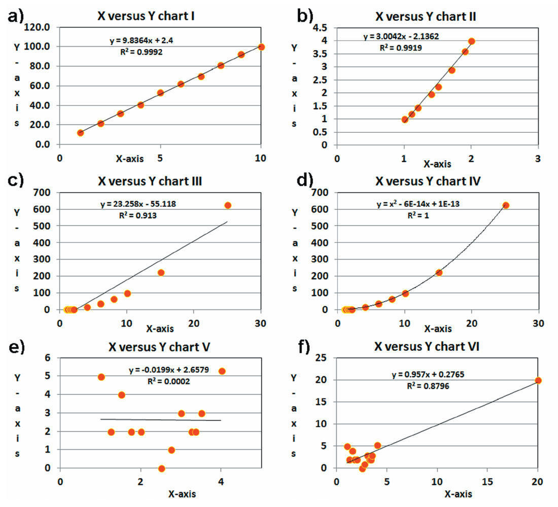
The y =10x solution of 1(a) has a near perfect correlation coefficient. Figure 1(b) is a portion of y=x². Despite the fact that the relationship is non-linear, the correlation coefficient is high and the regression line is a reasonable fit for this data range. Figure 1(c) is the same relationship for a bigger data range. There is some clear misfit, but the correlation coefficient is still quite high and the defined linear relationship is still fairly accurate within the data range. Figure 1(d) shows the same data as for 1(c), but uses a curvilinear regression fit (formula given) with a nearly perfect correlation coefficient. This is a better answer than the linear regression approach to a non-linear problem. The example does illustrate that we may choose a more appropriate model to fit non-linear relationships, or we may choose to live with the error of linear regression applied to non-linear problems. Statistical tests, such as the run statistic, exist to test the model fit, but observation alone indicates there is a problem with linear regression on the data of Figure 1(c). Figure 1(e) shows an attempt to correlate a random data relationship. Note that the 1% p-test is failed, as it should be, in this example. Figure 1(f) shows the same data as in 1(e) with the addition of one outlier point. The outlier point is sufficient to create a statistically significant correlation coefficient. This example shows that use of the correlation coefficient summary statistic alone is insufficient. The data must be examined for outliers.

A hypothetical production estimation problem: multivariate analysis

Multi-variate linear regression will often be useful for exploration geophysicists, since many of our problems involve more than one variable. In fact, single variable analysis may yield low correlation coefficients because no single variable alone may adequately describe all of the changes in the variable to be predicted. Put another way, single variables may not describe a significant amount of the variance by themselves. Let us consider a simple hypothetical example.

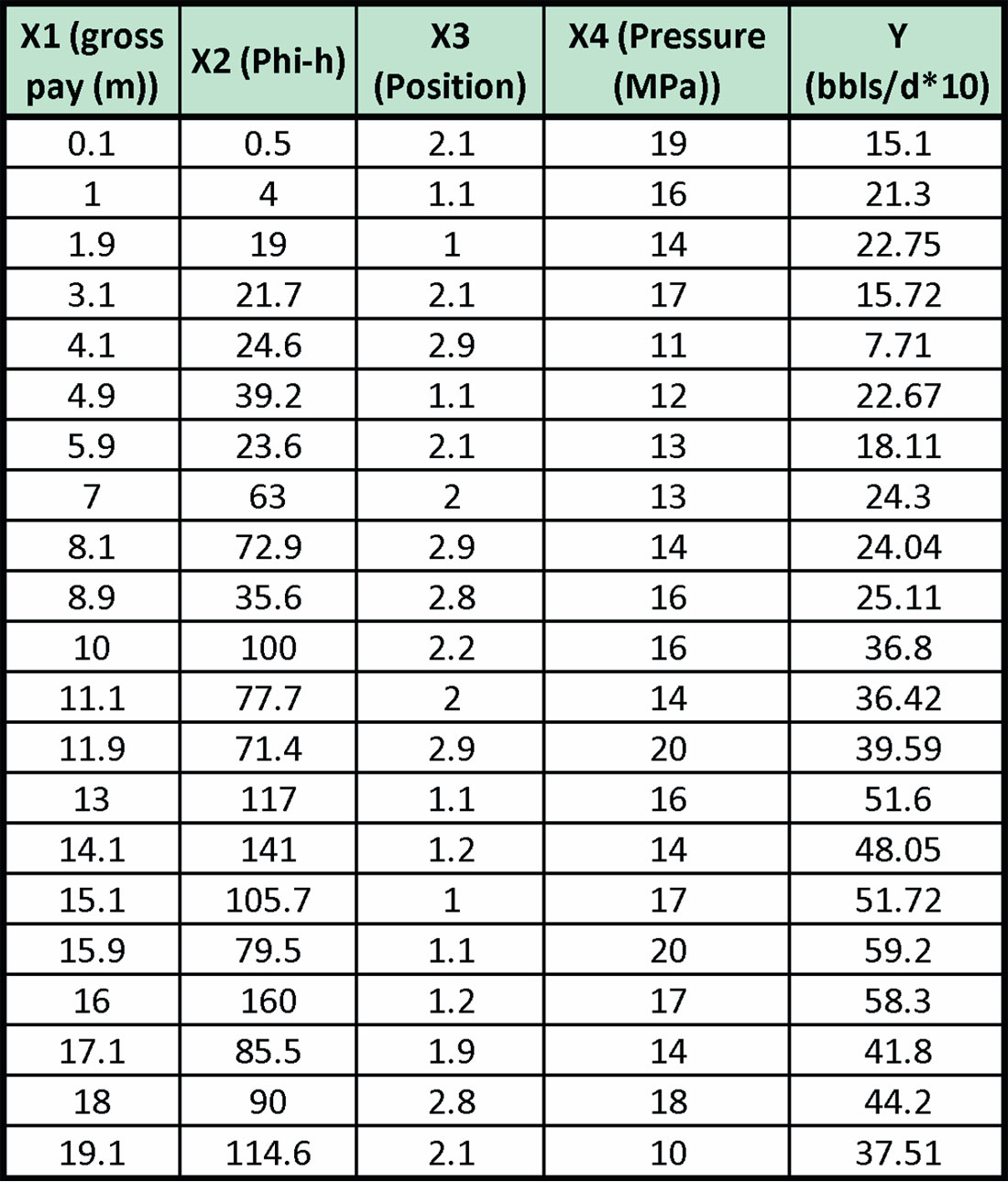
We are attempting to predict production (Y), which is measured in 10’s of barrels of oil per day from a marine barrier sand. We have four candidate variables, X1, X2, X3, and X4, which could be related to production. These variables have a potential relationship to production through Darcy’s law, although the relationship is not truly linear. The variables are defined as:

There are 21 samples (or wells). The data is given in Table 1.

The data was defined (or created) with the following relationship:

A small amount of noise has been added to the solution for Y (equation 9). We can attempt single variable linear regression for each of the X variables against Y individually or we can attempt a multi-variate regression involving all four of the X variables. Figure 2 shows the results of such an effort.

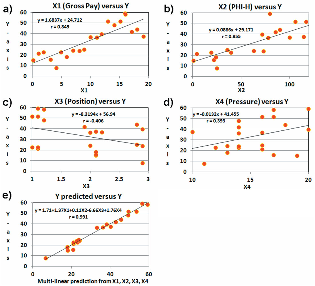
Given 21 samples, the 5% p-test requires a correlation coefficient of 0.433. Interestingly, both X3 (position) and X4 (pressure) fail the 5% p-test. Our prior knowledge of production may suggest that the problem is multi-variate and that pressure and position should be used in a multi-variate estimate despite their failure in the test for statistical significance. This is something that Fisher (1935) talks about: we should use all knowledge at our disposal. We must remember that we are testing a hypothesis based on physical expectations, and to a large sense this should drive our statistical testing. It is true that this can open us to confirmation bias, but it makes sense to use all the knowledge at our disposal, and that knowledge suggests we should look closer at X3, and X4 despite their failure.

With this in mind, we performed a multi-linear regression estimate of production using all the predictor variables. The solution was statistically significant in all variables. The multi-linear regression solution to this problem yields the following formula:

This estimate is close to the correct answer given in (9), but the weights are not quite correct.

The correctness of model is a concern with this multivariate approach to production prediction. Darcy’s law suggests that production behavior follows a multiplicative relationship between an area term, pressure draw-down, permeability, and one-over-viscosity. We have used a simple linear relationship to predict production. To some extent this was incorrect. We could have linearized Darcy’s law and applied our method, but we took our simple and somewhat incorrect approach. Why did we do this? We did it because it is simple and illustrative. At an early or immature state of enquiry, simplifying to a linear relationship can be an appropriate first step. It is very important to recognize that the method is not strictly correct, and not to forget that the approach is best treated as a temporary measure for an early purpose. At a later stage, the equation should be treated in a more correct manner. Note that multiplicative relationships can easily be linearized by taking the logarithm of the equation. This is a common procedure among statisticians that leads to log-normal distributions and should be used when appropriate during more advanced stages of analysis. This entire apology being said, I like the early use of multilinear regression because it is fast and the weights can test the physics (or hypothesis) underlying the problem. The weights of normalized variables can also illustrate, together with the correlation coefficient, which variables are dominant.

STEPWISE REGRESSION

Our multi-variate example was made straight forward by the fact that we had four predictor variables, and we had a priori reason to attempt combining them all. What happens when we have many more potential predictor variables and we are not as confident that they should all be used? What happens when we face the very real possibility of over-fitting our solution? How do we choose the variables we should use, the number of variables, and the order in which they should be used? We can attempt Step-Wise regression. To do this, we employ simple multilinear regression as defined by equation (5). The method is described as follows:

1. Test all variables for correlation coefficients with single variable regression.
2. Choose the single variable with the highest correlation coefficient. This variable, called the first variable and its regression formula define the best single variable prediction model.
3. Perform a p-test. If the p-test is passed, continue.
4. Perform two variable regression, using every combination of two variables possible. The two variables that give the highest correlation coefficient are chosen as the two variable solution. These two variables and their regression formula define the best two variable production prediction model.
5. Perform a p-test. If the p-test is passed, continue to the best three variable test.

This process continues until the p-test is failed. This method could be called an exhaustive forward step-wise regression. There are variations of the method that are less exhaustive which freeze the variables as they are chosen. In such a case the best single variable would automatically be one of the variables used in the two variable step. The two variables from the two variable step would be automatically used in the three variable solution. The less exhaustive techniques are not guaranteed to find the best solutions. Some caution is required with step-wise regression as it is quite easy to use too many variables. Justification of variables by hypothesis should be undertaken, as mentioned earlier. We should not use variables that we do not have reasonable justification for, or which are dependent on variables we are already using: this can cook the books! Additionally, there exist other tests (one of which we will discuss next) to help determine when too many variables have been used.

Let us test this method with our multi-variate example. We will use the same data from Table 1, except that we will add two variables to the data. Each of these two variables are range bound and random. They are not related to production (Y). The new data table is given below as Table 2.

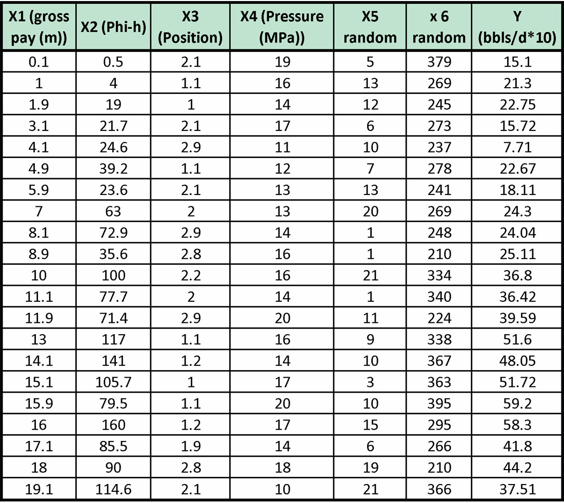
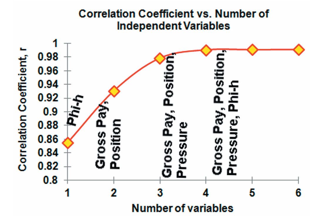
Using the step-wise regression procedure, we determine the best multivariate solutions. This analysis iss illustrated in Figure 3. The correlation coefficients rise through the first three variables. The best three variable solution is: gross pay, position, and pressure. The addition of Phi-h in the

four variable solution adds little to the correlation coefficient because of the degree of dependence between gross pay and Phi-h. The fifth and sixth variables to be added are X5 and X6, which we know have no relationship to production. These last two variables fail their multivariate p-test. The observation of the rate of change of the correlation coefficients in step-wise regresssion is informative to how many (and which) variables should be used in an optimal solution.

CROSS-VALIDATION TESTING

Another method of estimating the correct number of attributes to use in a multi-variate study is called cross-validation. The method differs from p-testing in that it evaluates the actual predictive capabilities of the regression formulae. The idea is to evaluate the effect of overtraining and outliers on the predictive solution by dividing the sample into two groups, one in which the multi-linear weights are calculated, and another, hidden group, upon which the weights are tested in a predictive fashion. The predictive error is calculated for the hidden group. The prediction error we calculate is the total error in prediction from equation (4) divided by the number of samples, making it an rms average of the error:

We express the results in terms of a percentage error from the sample mean of what is being predicted. Similarly to Hampson et al (2001), our method is a leave-one-out-cross-validation (LOOCV), which we employ in conjunction with step-wise regression. The method follows:

1. Take the best single variable.
2. Choose one element from the sample as the hidden group.
3. Calculate the regression weights using all samples except for the hidden group.
4. Use the regression formula to make the prediction for the hidden group.
5. Record the predicted value and the prediction error for the hidden group.
6. The hidden group goes back into the regular sample group and another element from the sample is chosen as the hidden group.
7. Repeat the calculation of regression weights with the new sample and apply them to predict the production of the new hidden group.
8. Record the predicted value and the prediction error for the new hidden group.
9. Repeat this process until all elements of the sample have been the hidden group one time.
10. Calculate the rms average prediction error for the single variable cross-validation test
11. Perform the same process for the best two variables from the step-wise regression analysis.
12. Calculate the rms average prediction error for the two variable cross-validation test
13. Continue this testing process for the best three variable solution, and so on.
14. Plot the rms average error versus the number of variables in the solution. When the error bottoms out, or its downward slope is significantly reduced, the optimum number of variables has potentially been found.

The predictive error calculated in formula (11) always decreases with increasing number of variables when the same sample is used for regression analysis and for prediction. With cross-validation, this is not the case. Prediction error calculated with our method of cross-validation will typically bottom out or reach minima when the number of variables in the solution is optimum (Hampson et al, 2001). Additionally, the regression weights are calculated n times, and can be examined for consistency. Please review Hampson et al (2001) for examples of the LOOCV method.

Conclusions

The tools of statistics are essential to the modern quantitative geophysicist. They represent an important part of an efficient and accurate experimental vocabulary. I have touched upon a few of those tools, and hinted at a few more. It is my hope that this column might encourage a deeper exploration into the language of quantitative methods.

Acknowledgement

I would like to thank the VIG Steering Committee for their help in reviewing this document.

References

Davis, J. C., 1986, Statistics and Data Analysis in Geology; John Wiley and Sons, Inc.

Fisher, R. A., 1935, The Design of Experiments (9th ed.). Macmillan

Gray, D, 2013, An Unconventional View of Geophysics: CSEG RECORDER, 38, 9, 50-54.

Hampson, D.P., J.S. Schuelke, and J.A. Quirein, 2001, Use of multiattribute transforms to predict log properties from seismic data: Geophysics, 66, 1, 220-236.

Hughes, W., J. Lavery, and K. Doran, 2010, Critical Thinking: an Introduction to the Basic Skills, sixth edition: Broadview Press.

Hunt, L., 2013a, Estimating the value of Geophysics: decision analysis: CSEG RECORDER, 38, 5, 40-47.

Hunt, L., 2013b, The importance of making conclusions and frameworks in reasoning: CSEG RECORDER, 38, 7, 56-60.

Kalkomey, C. T., 1997, Potential risks when using seismic attributes as predictors of reservoir properties: The Leading Edge, 16, 247-251.

Rodgers, J. L., W. A. Nicewander, 1988, Thirteen ways to look at the correlation coefficient: The American Statistician, 42, 1, 59-66.

Sokal, R. R., and F. J. Rohlf, 1995, Biometry, Third Edition, W. H. Freeman and Company.

Sterne, J. A. C., G. D. Smith, 2001, Sifting the evidence–what’s wrong with significance tests?: BMJ (Clinical research ed.) 322 (7280): 226–231. doi:10.1136/ bmj.322.7280.226

Wikel, K., 2013, The Future of Geomechanics And What It Means For Geophysics: CSEG Recorder, 38, 8, 60-62.