I came across a couple of interesting items related to recent Science Break articles. On circadian rhythms (December 2013 RECORDER) I read about a company which offers a clock that, “monitors sleep patterns… and uses coloured lights customized to your circadian rhythms to facilitate sleep, and to wake you at an optimal time.” (National Post, 2014) To find out more, Google “Aura clock”.
On encryption (June 2013 RECORDER) a recent Economist article (The Economist, 2014) describes how researchers are getting close to deciphering encrypted computer messages, in a most unexpected way. They have been able to listen to computers – literally listen to the sonic vibrations – and identify a unique signature for each RSA encryption key. To identify which key each signature belongs to, they get the computer to decode known messages, thus tricking it into revealing its codes. Interestingly, one of the researchers is Adi Shamir – the S in RSA cryptography refers to his last name – so he is working on rendering his own encryption technology, developed many years ago, obsolete.
Electrical and Electromagnetic Survey Methods
This recent January I started a new phase of my career when I joined Quantec Geoscience Ltd. Quantec specializes in ground-based electrical and electromagnetic geophysical surveys, methods which I studied (not very well) three decades ago and subsequently forgot. As a way of forcing myself to get conversant in these methods as quickly as possible, I publicly committed to writing a Science Break article on them, which I immediately regretted. I suppose that foolish promise worked, although it did result in three missed months of Science Break. At any rate the following article captures my grasp of the topic at the current time. What I have found is that there has been a remarkable advance in these technologies, which is hardly surprising when I think of all the advances in seismic over the same period. Full disclosure: I have written this article with co-author and colleague Darcy McGill, along with assistance from Kevin Killin; both are experts in this field (of fields).
Electrical Methods
Electrical geophysical methods measure only properties related to the electrical field, most often by directly measuring potentials (voltages) in the ground. As such, electrical methods are generally ground- or borehole-based, and measure responses from the earth which are governed by Ohm’s Law.
SELF-POTENTIAL (SP)
Sometimes called spontaneous potential, this electrical method is a passive technique that involves simply measuring the natural potentials in the earth. In the oil patch SP is commonly measured as a way to make inferences about lithology. The potential being measured is usually caused by differential movement of ions between the zone invaded by fresh water drilling mud and the virgin rock; in permeable zones, the measured SP response is largely a function of the volume of water in the pores and its salinity, and the amount of clay present in the pores.
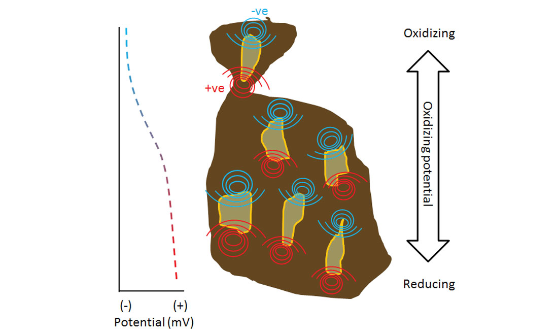
In the mineral sector the SP method has been used extensively since its invention in 1931 by the Schlumberger brothers. There is an active debate in technical circles around the cause of SP anomalies measured over massive sulphide ore bodies. The long accepted dipole theory posits that differences in oxidization potential between the top and bottom of the ore body cause electrons within the body to move from one end to the other, and this creates a return current in the surrounding rock. However, this explanation is problematic because measured SP responses routinely exceed 750 mV, the accepted upper limit for SP created by a dipole effect. The more recent redox theory is gaining credibility (Figure 1) (Hamilton, Hattori, & Brauneder, 2008). This model explains that if the ore body is held within a strong redox gradient (i.e. a strong reduction effect at one end grading into a strong oxidization effect at the other), then the ore body will become polarized, with a negative pole forming at the oxidizing end. This polarization will create a small SP effect within each mineral grain; grains that are end-on-end will tend to act as a multitude of little batteries in series, thus explaining the high potentials measured.
Mise-A-La-Masse
This is another simple technique dating back to the early 20th century, but it is an active method requiring an electrical source. It is used to delineate known electrically conductive bodies. Obviously this is useful; for example, if a mining quality ore body is discovered near the surface, then the next step is to determine the size and extent of that body.
One transmitter source electrode is located within the known conductor, either at the surface or at depth in a drill hole, and the other is located at electrical infinity. That sounds like a far way away, but in practice all that is required is a distance of at least 5 times the maximum expected dimension of the ore body. When the current is applied, the conductive body acts as an electrode of sorts, with current radiating from the entire ore body. Using two mobile probes hooked up to a voltmeter, the lines of equipotential can be mapped by the geophysicist, and these lines crudely reflect the actual shape of the ore body. Mise-a-la-masse can be used on the surface, but is often used to detect the continuity of conductive mineralization between drill holes. Other applications include delineation of other types of conductive bodies, zones or features, such as old pipes, flooded mine shafts, leachate plumes, and mineralized fault zones.
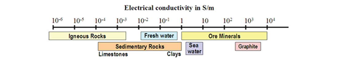
The physical property being measured is, obviously, resistivity; the lower a material’s resistivity is, the easier it is for an electrical current to pass through it. The key physical parameters determining resistivity are rock type, porosity, permeability, saturation porosity, the concentration of dissolved solids in the pore fluids, and the metallic content of the solid matrix. The following chart gives typical resistivity ranges for what we find in the subsurface.
It is important to distinguish between resistance and resistivity. The actual ease or difficulty with which a current flows through a body of a certain material is obviously also dependent on the geometry of the body, in addition to its physical properties as listed in the previous paragraph. A current flowing through a very thin wire will experience greater resistance than it would flowing through an identical wire of much larger diameter. What we want to measure is resistivity, which takes the physical dimensions of the body out of the equation, in other words resistance per unit volume of material. Ohm’s Law defines resistance as Potential/Current, or Volts/Amperes (V/A) measured in ohms. So resistivity is defined as the voltage across a unit length (Volts/metre (V/m)) divided by the current flowing across a unit area (amperes per square metre (A/m2)). This gives the resistivity, resistance per cubic metre, which is typically given the symbol rho or ρ, measured in units of ohm-metres, or Ω · m.
DC Resistivity/Induced Polarization (DCIP)
DCIP is another active method that measures both the resistivity of the earth by relating the current injected into the ground directly to measured potentials at the receivers, and also the chargeability by measuring the transient response after the injection current is switched on or off. What this means in practice is that two forms of survey can be conducted by the same crew and equipment – the traditional DC resistivity survey as described in the previous section, and the more modern time series IP survey.
You’ll have to indulge me as I go off on a time series tangent. I don’t believe these methods were taught when I was in university – I think all we were exposed to involved instantaneous measurements of electric and EM fields – but using time series data is now a key aspect of mineral exploration. When I first visited Quantec’s operations warehouse in Toronto I was amazed at how similar it looked to a seismic warehouse. There were the usual trucks, dog houses, and assorted field gear; lots and lots of cable; a big metallic box the size of a shipping container; and most interesting, stacks of boxes that looked exactly like seismic recording units. Turns out they are essentially repurposed seismic recording boxes. (The big metal box is a Faraday cage used to calibrate the magnetic receiver coils.)
The mining exploration sector is dwarfed by the seismic industry, so geophysical mineral exploration equipment advances have tended to follow those of seismic instrumentation. When the first networked, 24-bit seismic systems based on the delta-sigma chip first appeared, companies on the mineral exploration side were quick to see opportunities. Various companies came out with systems capable of recording digital time series data, and there was an explosion of advances around the time series recording of electrical and EM data.
Since many economic sulphide minerals are chargeable, DCIP is an important and commonly used tool for near-surface (down to ~1000m depth) mineral exploration. Depth of penetration is a function of geology and system configuration. A highly conductive layer tends to prevent penetration to rocks below, similar to how highly reflective layers in seismic hamper penetration of signal to depth.
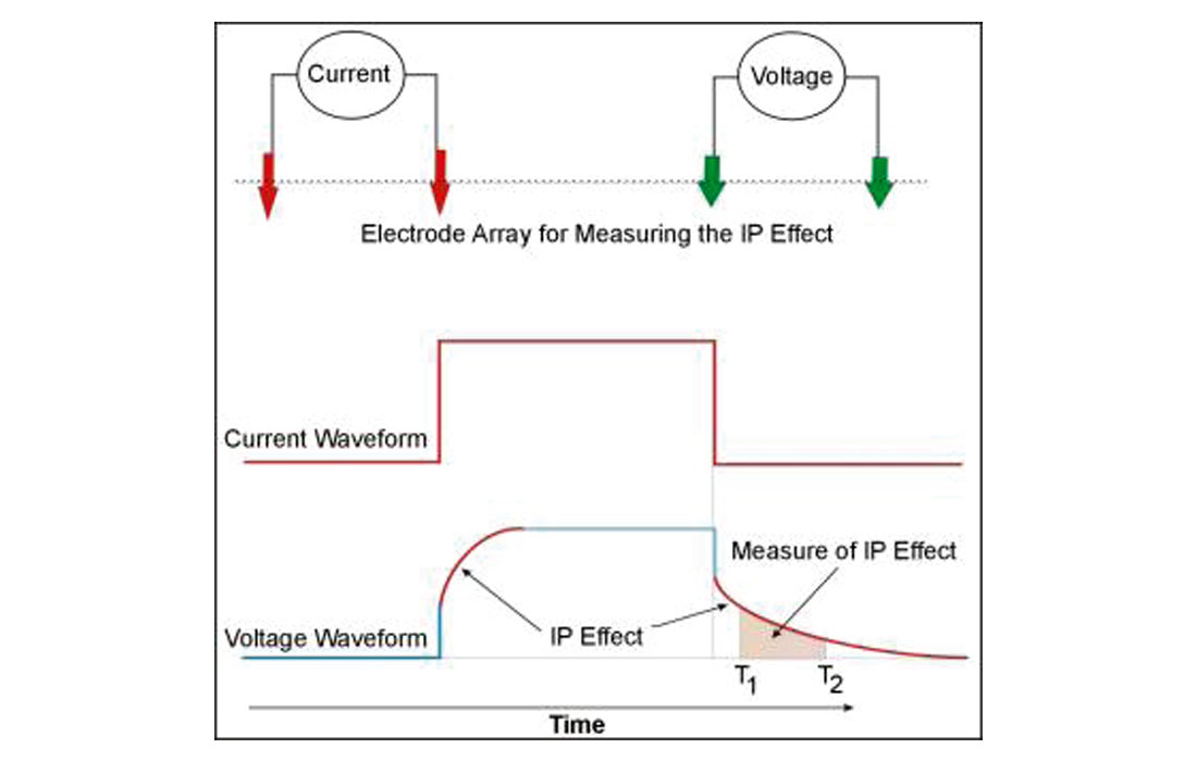
How IP works is like this. The crew injects the current into the ground with the source electrodes, and then turns it off. The receiver electrodes measure the voltage response over time, recording how the rock charges up and then briefly holds the charge (Figure 4); this response, a function of the level of polarization at rock interfaces, tells us something about its composition. What happens at these interfaces is a current-induced transfer of electrons between electrolyte ions and certain minerals, especially metallic-luster ones. With massive sulphides, it is the conductive sulphides reacting with the insulative rock matrix. In sedimentary basins, it is typically the clay content driving the IP effect, with other variables such as moisture content, rock / soil type, permeability, and porosity all coming into play.
How IP works is like this. The crew injects the current into the ground with the source electrodes, and then turns it off. The receiver electrodes measure the voltage response over time, recording how the rock charges up and then briefly holds the charge (Figure 4); this response, a function of the level of polarization at rock interfaces, tells us something about its composition. What happens at these interfaces is a current-induced transfer of electrons between electrolyte ions and certain minerals, especially metallic-luster ones. With massive sulphides, it is the conductive sulphides reacting with the insulative rock matrix. In sedimentary basins, it is typically the clay content driving the IP effect, with other variables such as moisture content, rock / soil type, permeability, and porosity all coming into play.
The actual resistivity measurement is derived by integrating the recorded voltage over time. Further nuances in composition can be gained by the use of frequency domain IP. This term is a bit misleading – the method doesn’t really use the frequency domain, rather it uses an AC current, repeats the experiment at different AC frequencies, and then compares how the IP response in the form of apparent resistivity varies versus source frequency.
Once the resistivity measurements are in hand, then the next step is to invert the data, and this is usually referred to as interpretation. I won’t go into what it involves as readers will be familiar with inversion, but essentially an earth model is chosen as a starting point, and then the computers grind away and reduce an error function to produce a final model. Figure 5 shows a typical ore body model derived via this methodology.
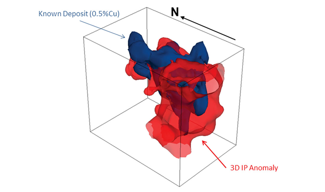
The example shown in Figure 5 is interesting. The blue body represents the best estimate of the iron oxide copper gold (IOCG) ore body’s geometry prior to the survey, based on what had already been delineated by drilling; the red represents the result of the geophysical survey. Subsequent drilling confirmed the accuracy of the geophysical image, and this resulted in millions of dollars more ore being discovered. The differences between the red and blue models up shallow are easily explained – the ore here is weathered and oxidized, meaning there was a greatly reduced IP response. Note that this result was achieved by jointly inverting DCIP and MT data, a specialty of Quantec’s that provides continuous results from shallow to deep.
Electromagnetic Methods
Electromagnetic (EM) geophysical methods measure properties related to both the electric and magnetic fields to map resistivity. EM methods rely on responses in the earth generated by electromagnetic induction using time-varying electromagnetic fields. EM methods are used both on the ground and from the air. In general EM methods measure responses from the earth governed by Maxwell’s equations. As with seismic, lower EM frequencies penetrate deeper into the earth. Also analogous to seismic, EM methods may be broadly grouped into passive and active methods:
Passive Methods
Magnetotellurics (MT)
Of all the methods I’ve been exposed to so far, I definitely find MT the most fascinating and intriguing. It relies on natural source fields (solar-magnetospheric interaction for lower frequencies, and global lightning activity for higher frequencies). The electric and magnetic fields are measured independently, and the relationship between them is used to calculate the resistivity of the earth. MT is able to measure extremely low EM frequencies (often 0.001 Hz or lower), and is thus able to estimate resistivities to great depth. This obviously is important, since the active methods are limited to relatively shallow exploration. Because of this, receivers record for long periods of time; the deeper the investigation, the lower the frequencies of interest, hence the longer the recording time. For typical mining and geothermal projects recording time is 10 to 16 hours, but the longest I’ve seen so far was 36 continuous hours. As with the other resistivity methods, the data are then inverted. This is a complex and computationally intensive process, increasingly so with depth and size of survey, exponentially so for 3D projects.
MT is used for a variety of applications, including deep continental-scale crustal investigation to depths of tens of kilometres or more, geothermal exploration to identify the location and extent of the heat “reservoir”, and of course deeper mineral exploration (often used to map large-scale deep-seated mineralized systems like copper porphyry deposits). Similar to oil & gas, there are fewer near-surface minerals left to find, so the mining industry has been forced to search for ever deeper deposits, meaning MT technology is becoming increasingly important.
Controlled Source Audio MT (CSAMT)
CSAMT is measured like passive MT but uses a dipole transmitter located several km from the survey area to generate the signal for the survey. CSAMT uses frequencies in the audio range (approximately 1-10 kHz) and is thus a much shallower penetrating technique than passive MT.
VLF-EM
VLF is a semi-passive (sounds like many geophysicists) method that relies on VLF transmitters (15-25 kHz range) around the world for its signal. VLF has fallen out of favour somewhat in recent times; it is a shallow-penetrating method sensitive to overburden, and also sensitive to the direction of the source transmitters. Also, many VLF transmitters around the world have been shut down due to modern communications systems crowding those frequency bands.
Airborne Passive Systems
Passive EM from the air presents a number of challenges; it is currently not practical to measure the electric field, so systems such as Geotech’s ZTEM measure only the vertical component of the magnetic field. The airborne measurements are combined with measurements of the horizontal components of the magnetic field from a fixed base station to produce what is known as “tipper” data.
Active Methods
Active EM methods are grouped in to two classes, frequency-domain and time-domain.
Frequency domain EM (FDEM) uses transmitters that transmit constant signal on specific frequencies, and receivers that are tuned to the same frequencies. The measured resistivity is related to the phase shift between transmitter and receiver. Time domain EM (TDEM) systems transmit pulses of energy and measure the transient response of the earth. Resistivity is related to the decay of the induced signal in the earth during the transmitter off-time. Some systems can also measure during the transmitter on-time.
Airborne EM systems are used for large-scale regional mapping, as well as mineral exploration on various scales. EM is also used for environmental and engineering mapping, as well as shallow petroleum exploration (oil sands, mapping palaeochannels, etc.)
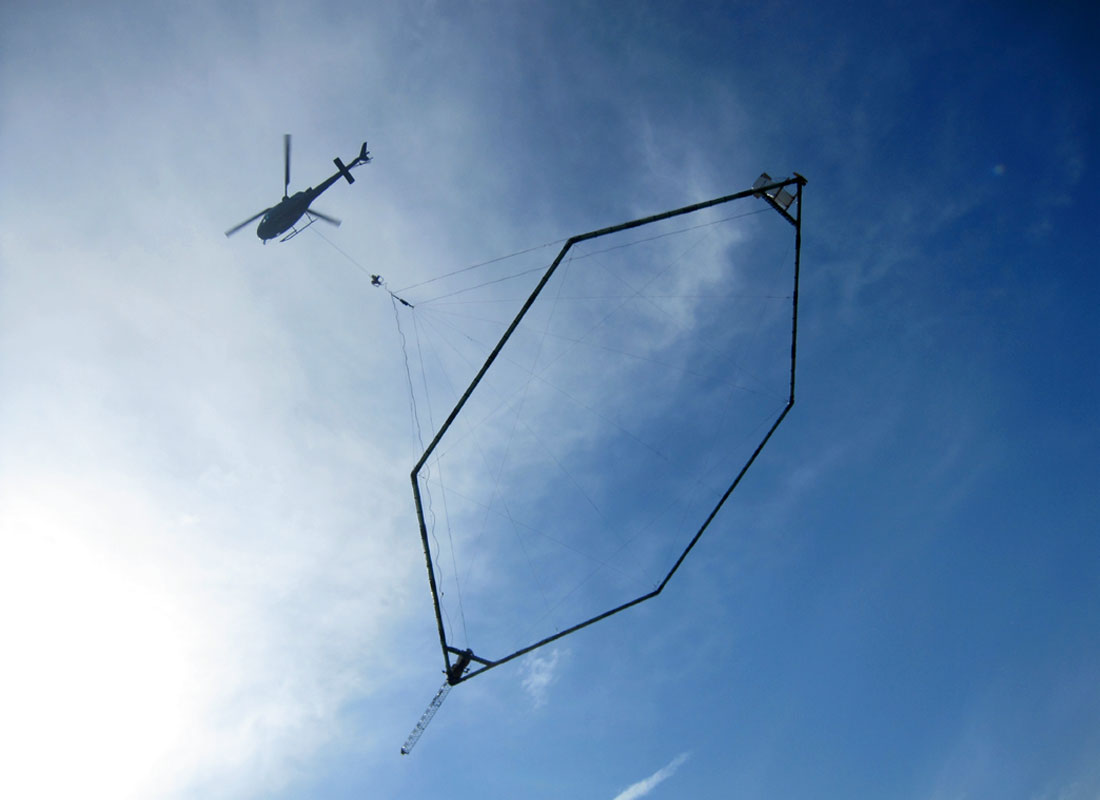
Typically, airborne TDEM systems are deeper-penetrating and offer lower resolution than FDEM systems, but there exist considerable differences in the technologies available. Unlike seismic companies which more or less offer the same final product, and are differentiated on capacity, location, cost and other non-scientific criteria, in the electrical survey world the technology can vary significantly between companies. For example, one company, SkyTEM, offers a helicopter- based form of TDEM that uses a dual-moment capability to map both shallow and deep geology, concurrently and in high resolution (Figure 6). This means they can tailor their surveys to the type and depth of target.
There is also a large range of ground EM systems, both FDEM and TDEM. Large-loop ground TDEM systems allow deep measurements using lower transmitter base frequencies. Ground EM systems are used on smaller scales for target definition in mineral exploration. Borehole EM systems allow the direct measurement of the geometry of conductors down hole, and are an important tool for defining ore bodies.
Electrical Methods and the Oil & Gas Sector
CSEG readers that have persevered this far are probably asking, “What’s in this for me?” Well, this may not be indicative of anything, but recently Quantec has seen an uptick in interest from the petroleum industry. I get the impression that there have been previous periods of interest from the oil & gas sector in the electrical methods, which then faded when results fell short of expectations. Seismic is so ideally suited to exploring hydrocarbon rich sedimentary basins that it is hard not to be disappointed by other methods. When compared with seismic, resistivity data are very low resolution. However, the lure of somehow complementing seismic methods with electric data is compelling, as there are many situations where seismic struggles, for example in areas with near surface volcanics or permafrost. And shouldn’t there be some advantages to bringing in different types of information, especially resistivity which is a property measured in almost every well log?
Water is really at the heart of most situations that may be helped with the addition of resistivity data. The presence of any kind of water lowers resistance, and there is also a difference in resistivity between fresh water and saline water. This holds the promise that electrical / EM methods may be useful in applications such as steam flood monitoring, fracture detection, and detection of ground water contamination. I see the use of resistivity data in oil & gas applications falling into two categories – first, to aid the modeling of the near surface and thus improve static calculation and possibly velocity model building i.e. a complement to processing; second, as an additional form of data down at the actual zone of interest, i.e. a complement to interpretation.
To help out processing, I see shallow resistivity measurements (such as from DCIP surveys) being incorporated into the refraction solution, probably via joint tomographic inversion or something like that. This could/should result in image improvements, but I’m skeptical whether this would be enough for an oil company geophysicist to loosen the purse strings, especially since it would involve significant additional costs to run a resistivity survey, all just to improve statics a bit.
Incorporating resistivity data, probably MT data, at the interpretation stage on the other hand, I could see catching on. There have been some examples in the literature and advertising propaganda of joint seismic / resistivity inversions (I have included some good papers on this general topic in the references below.) These inversions either rely on relationships between resistivity and some seismically derived value, such as those described by the Faust or time average methods. Alternatively, approaches exist that involve a sort of back and forth exchange of resistivity-derived boundaries with reflectivity-derived boundaries converging on a joint solution; another approach – and I’m really simplifying here – involves a similar back and forth iterative approach, but at the parameter level – data driven automatically derived empirical relations are found by the software, resulting in a convergence on a solution that marries the seismic and the resistivity data.
I can think of two situations (I’m sure there are others) where the additional cost of acquiring resistivity measurements along with seismic could be justified, assuming the results were of sufficient quality. The first involves a common situation in heavily structured areas. Often underneath outcrops, especially weathered/karsted carbonates, almost no coherent seismic data is recorded. This forces interpreters to make inferences and other educated guesses. In cases like this, resistivity data could at least give an understanding of the basic geometry of the structures – faults, synclines, anticlines – information that is far better than none at all. The second situation involves areas where seismic quality is good, but there is a risk of structural traps being wet. In cases like this, with the traps clearly defined by seismic, the resistivity data, even if blurry and blob like, could give an indication whether there was oil or water in a trap; with the cost of deep wells in some areas, the economics could make sense.
My buddy Dave Gray feels that incorporating resistivity data into a geostatistical solution is a better way to go, and I tend to agree with him (I’m very easily swayed by people who are smarter than me). Resistivity is a physical property that is entirely independent from seismic, so surely an improvement over adding yet another property derived from seismic amplitude to the statistical stew. When I sit through some of these seismic geostatistics talks I feel like I’m a guest at a hillbilly wedding. A while back I was editing the CREWES 25th anniversary RECORDER interview, and I noted that Rob Stewart, when asked about the future direction of research and advancements, mentioned that he felt that the incorporation of other physical measurements along with seismic is an area that warrants further research and offers some promise. Perhaps that’s a sign that I’m not out to lunch.
Key Search Acronyms
EM, MT, IP, DCIP, TDEM, FDEM, Faust equation, joint inversion


Share This Column