Expert Answers

Question

In processing of seismic data a surface consistent approach assumes that the basic wavelet shape depends on the source and receiver locations and not on the raypath separating the two. So, for a surface consistent formulation, a seismic trace is usually decomposed into the convolutional effects of source, receiver, offset and the earth’s impulse response. Such a formulation has been used fruitfully for statics application, deconvolution and scaling of land seismic data. Surface consistent approach is also useful for AVO analysis.

Please comment on the application of a surface consistent approach to marine seismic data or seismic data from transition zones. Your answer is expected to include:

1. If such an approach is commonly used for marine data, and if not, then why not?
2. Where is such an approach most useful and why?
3. What types of differences can be expected on the data with surface consistent application? Please use real data examples to illustrate your answers.

Answer

Surface-consistent processing is just that: analyses and corrections designed to remove the effects of variable source and receiver responses. We take advantage of the typical near-vertical surface ray-paths (due to ray-bending) to strip out the near-surface effects on our imaging (amplitudes, phase, statics), lumping them all in together into a surface position tied to a source or receiver location. Let’s now look at the question concerning the relevancy of surface-consistency to seismic marine data processing.

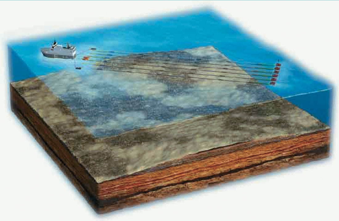
I’d first like to point out that marine acquisition (and therefore, its data) is a rather lucky, special case. To generalize, marine sources (typically tuned air gun arrays) and receivers (hydrophones embedded in solid or oil-filled cables) are towed in the water behind a vessel at depths typically 4 to12 m below the surface. My example (Figure 12) has two guns and six streamers/cables. From a land-locked Calgarian’s point of view, why is this significant? What’s noticeable right off the bat is that there is of course no true “surface-consistency” for these receivers, since they are always moving, being towed along smoothly throughout the entire acquisition. “Feathering” (sideways receiver drift caused by currents and boat directional changes) adds an even bigger challenge to the whole concept. What we therefore choose to do is to “bin” receivers to an assigned surface grid (a bit like the way CMPs are binned in a land 3D). The source locations are all unique, and therefore pose no problems here. In fact, each source is incredibly consistent, shot to shot, sail line to sail line. The receivers can remain physically the same units throughout an entire group of marine surveys (barring the odd shark attack and the like). Another bit of information: there is nearly perfect coupling and virtually no coupling variation from one part of a marine survey to the next - either for source or receiver. On land, we of course have the opposite scenario, causing much of the image distortions through delays, attenuation, and phase variations. The only such effects in a marine environment are those due to water velocity (temperature and salinity) and tidal variations, and these can be dealt with in a surface-consistent manner (although they are more sail-line consistent than shot-consistent).

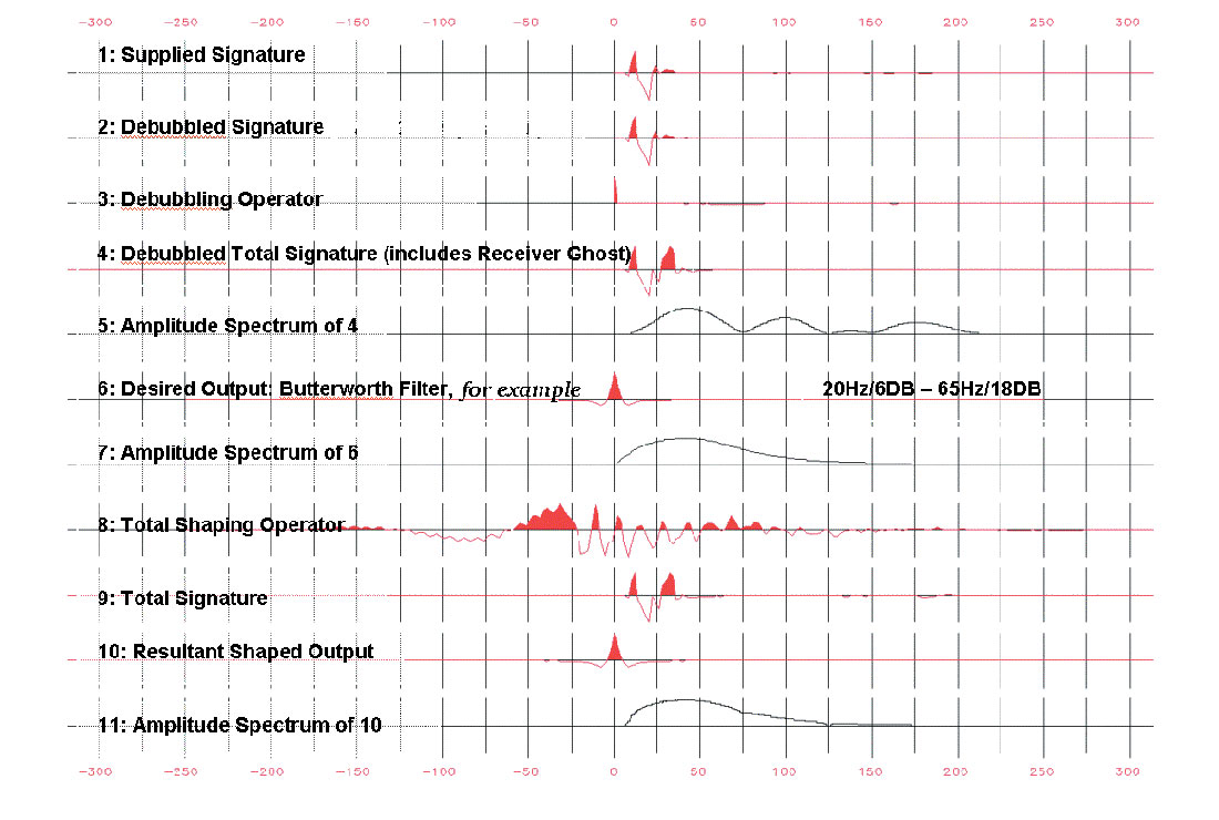
To sum up, a modern marine data set will have a very consistent source and receiver response – something that could never exist in a land data set. Recognizing this, the industry has, relatively recently, adopted as a standard, “deterministic” deconvolution (as opposed to the more commonly recognized “statistical” version). The steps of this approach are really straightforward and similar to the “Model-Based Wavelet Processing” of the 1980s, typically involving a farfield source signature, some modeling of acquisition effects, and aiming for one global operator to reshape the total model to a specified (zero phase) output. The more complex marine acquisition styles like wide-azimuth (and OBS) will require a directivity correction as well. A simplified example of this derivation is summarized in Figure 13.

In this newer approach, no wavelet-compressing, statistically- derived Weiner-Levinson deconvolution should be applied. The deterministic results are generally fantastic, with a phase-consistency impossible to derive any other way. The point is important enough to belabor: rarely is the signal consistently well-sampled in any deconvolution design window, which is typically saturated with multiples that, in the marine world, come and go and are often more than 30 dB stronger than the primaries. There will always be some geological and signal variation in any deconvolution design window, distorting the resultant W- L deconvolution operators. In general, you’ll no longer see a “normal” five-term surface-consistent deconvolution applied to any marine data.

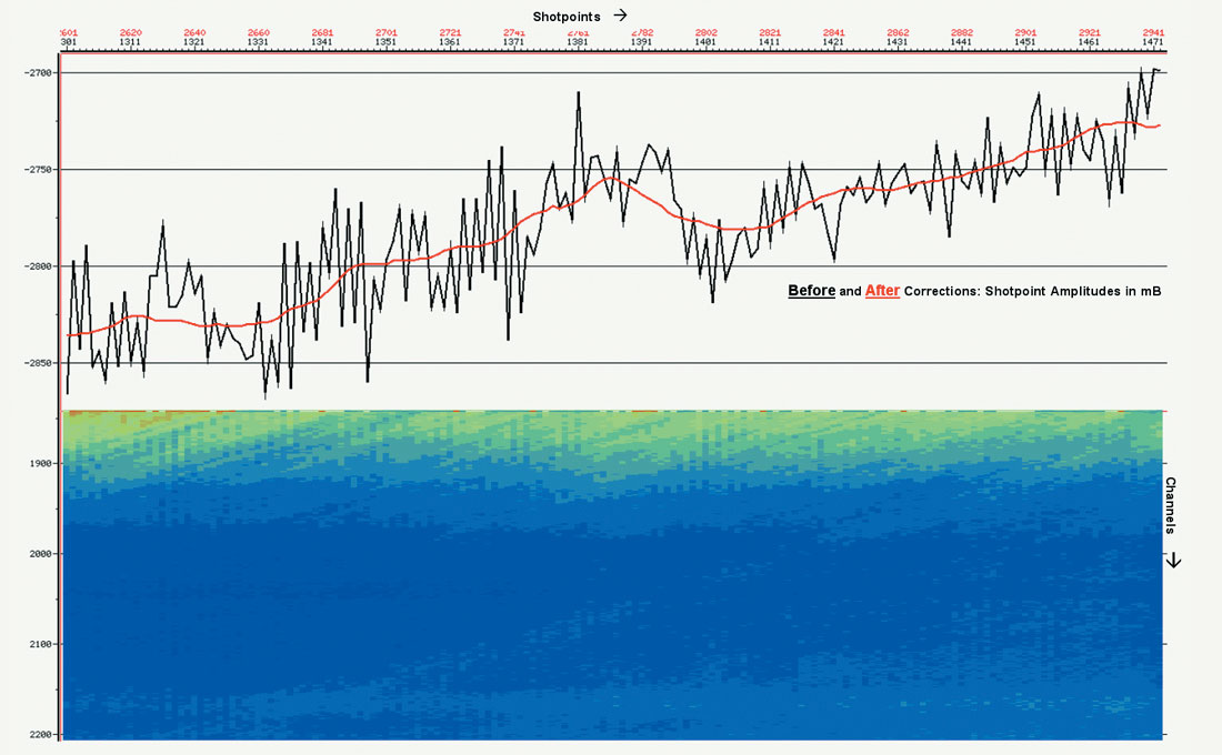
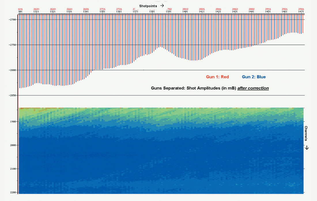
Let’s now look into marine amplitudes. For typical marine acquisition, continuous and expensive onboard QC keeps the source output to close tolerances, and, as said, the same physical receivers are dragged throughout the survey. Marine “surface-consistent” (amplitude) corrections tend to be defined a bit differently than the land case, therefore, instead of source- and receiver-consistent corrections, source- and channel- number- (effectively offset) consistent corrections are derived. In fact, only short-period amplitude variations should be addressed , adjusting the odd shot or channel (remember that perfect coupling...). At the same time, the small discrepancies between any of the multiple sources (“gun 1” vs. “gun 2”) can be removed. All of these corrections are normally small, very small – on the order of 0.2dB. Sail-line to sail-line variations are also normally in this range. Just as we saw in the decon situation above, a true conjugate-gradient/Gauss-Seidel 3D surface-consistent amplitude correction will normally do more harm than good. Figures 14 and 15 demonstrate a “typical” amplitude QC of a 3D marine sail-line.

Okay, so in theory things look a little grim for surface-consistent processing in the marine world. With the application of the above two “modern” (non-surface-consistent) approaches, most marine data becomes ideal in terms of phase and amplitude. Then, less manipulation is required in processing. And the less manipulation in processing, the more accurate our resulting image.

In practice, however, there are a whole slew of scenarios where surface-consistent processes work well. For instance, as long as the predictive gap is longer than our embedded wavelet, something like surface-consistent predictive decon can be an excellent tool for multiple suppression. And spiking surface-consistent decon can produce impressive results when applied to deepwater site surveys. As for amplitudes, strong geological variations just below the sea floor will require the more “typical” surface-consistent amplitude corrections. Here, we’re trying to remove amplitude footprints that are worse than any distortions introduced by a statistical approach. Of course, this would still require a first pass of the amplitude corrections described above.

Surface-consistent statics can also play an important role in marine processing. For instance, in the Beaufort Sea, variability in the waterbottom’s frozen layer can introduce fairly large distortions. Both tomo-statics and auto-statics can easily fix these (normally short-wavelength) problems. Surface-consistent statics can also play an important role in deep water seismic.

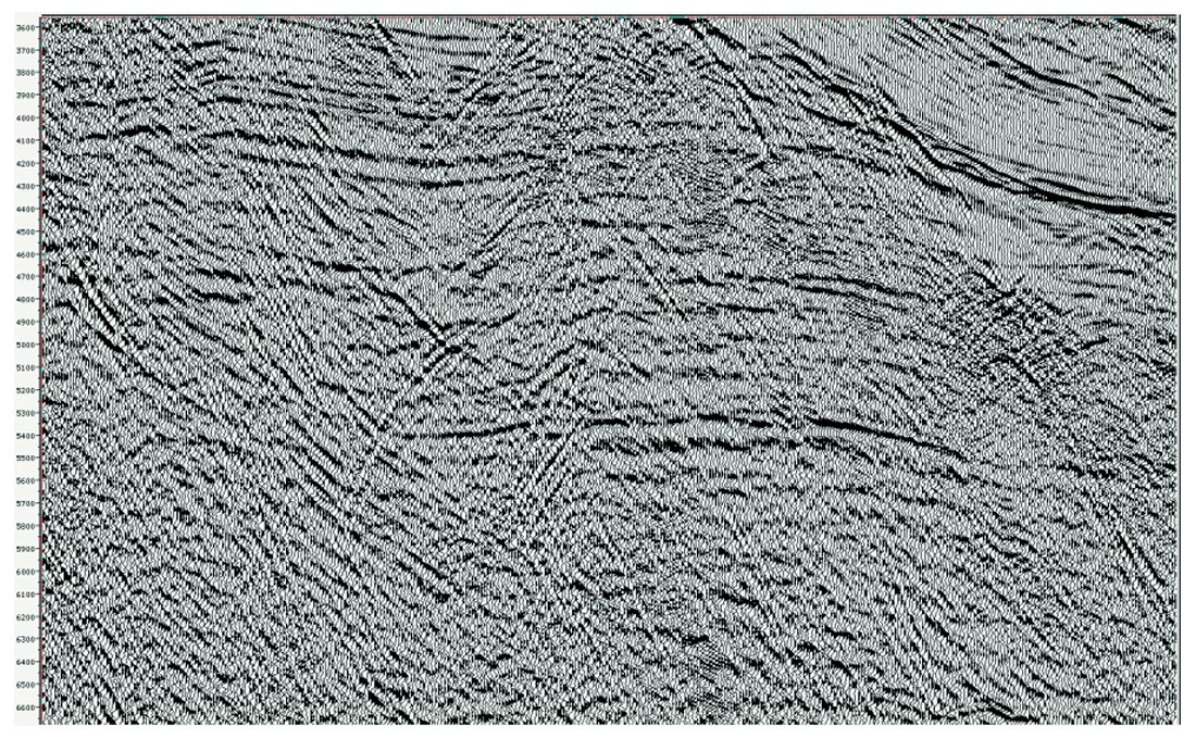
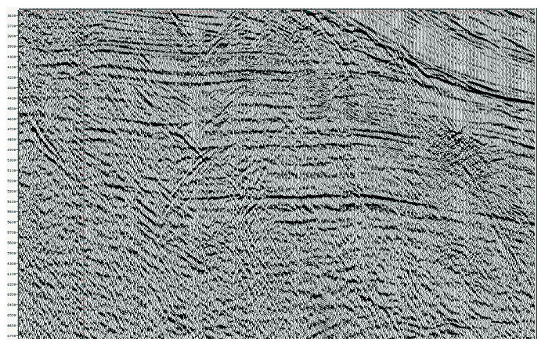
Turbidite channeling can cause some amazing waterbottom rugosity, giving us the same kinds of issues that a weathering layer in land would show. East Coast Canada marine data is full of these problems. This really requires PreSDM for a true fix, of course. For time imaging, however, a fairly robust solution can be derived through the use of surface-consistent modeling statics (Figure 16). In these cases, the statics don’t just improve the look of the section, they also create more consistent CMP gathers, allowing for better moveout, Radon demultiple, and so on.

And, I’ll save the most common surface-consistent marine practice for last: Surface-Related Multiple Elimination (SRME). SRME, introduced by Delft University of Technology, is a way of “automatically” predicting (and attenuating) multiples directly from the data itself. In fact, the SRME modeling process can be thought of as a surface-consistent auto-convolution. This powerful tool has become an industry standard in its 2D implementation for marine surveys throughout the world, and is becoming widely adopted in its 3D implementation.

Todd Mojesky,
CGG Veritas, Calgary

Acknowledgements

Thanks to BP, ConocoPhillips, Encana, ENI, Esso Exploration, Statoil, Norge, Norsk Hydro, Petoro, PetroCanada, and Total for many of the above (previously published) images. And special thanks to my colleagues at CGGVeritas for their invaluable reviews of my initial drafts.

References

Taner and Koehler, 1981, Surface consistent corrections, Geophysics, Volume 46, Issue 1, pp. 17-22

Jovanovich, Sumner, and Akins-Easterlin, 1983, Ghosting and marine signature deconvolution: A prerequisite for detailed seismic interpretation, Geophysics, Volume 48, Issue 11, pp. 1468-1485

Barr and Sanders, 1989, Attenuation of water-column Reverberations using pressure and velocity detectors in a water-bottom cable, Expanded Abstracts 59th Annual SEG Meeting, 653-656

Dragoset and Barr, 1994, Ocean-bottom cable dual-sensor scaling, Expanded Abstracts 64th Annual SEG Meeting, 857-860

Soubaras, 1996, Ocean-bottom hydrophone and geophone processing, Expanded Abstracts 66th Annual SEG Meeting, 23-26

Soubaras., 1998, Multiple attenuation and P-S decomposition of multicomponent ocean-bottom data, Expanded Abstracts 68th Annual SEG Meeting1336-1339.

Gratacos, et al, 2002, Calibration of horizontal components in the presence of azimuthal anisotropy, Expanded Abstracts 72nd Annual SEG Meeting, 971-974

Kommedal et al., 2002, Processing the Hod 3D multicomponent OBS survey, comparing parallel and orthogonal acquisition geometries, TLE, Aug, 795-801

Dariu, Garotta, and Granger, 2003, Simultaneous inversion of PP and PS wave AVO/AVA data using simulated annealing, Expanded Abstracts 73th Annual SEG Meeting, 63-66

Nordby and Gratacos, 2004, Vector fidelity correction for non-gimballed acquisition over the heidrun oil & gas field, Expanded Abstracts 66th Annual EAGE Meeting

Pica, Manin, Granger, Marin, Suaudeau, David, Poulain, and Herrmann, 2006, 3D SRME on OBS data using waveform multiple modeling, Expanded Abstracts 76th Annual SEG Meeting, 2659-2663

Ceragioli, Kabbej, Carballo, and Marin, 2006, Filling the gap: Nodes and streamer data are integrated for geophysical monitoring over a deepwater FPSO installation, First Break Volume 24, Dec, 49-53