Expert Answers

Question 1

Inelastic attenuation in seismic data is frequency dependent (higher frequencies getting preferentially absorbed) and increases with traveltime, altering both the amplitude and phase of the data. While processing for AVO analysis, attempts are made to remove the effect of the many factors that influence AVO response, so that the resulting amplitudes can be used to decipher geology. It is believed by some practitioners that offset-dependent correction for inelastic attenuation is not amplitude friendly, and so should be avoided. Others talk in favor of such a correction.

In your expert opinion, (1) What is your take on this? (2) Are we able to do an effective job of applying an offset- dependent inelastic attenuation to seismic gathers? If yes, how do you recommend applying such a correction – amplitude and phase, or only phase? Why? (3) What are the different techniques /methods available for applying such a correction? You may briefly describe each.

Question 2

Propagation of seismic waves through an overburden consisting of thin layers leads to transmission and interference effects, which need to be corrected for accurate AVO analysis. Amplitude and phase effects of fine layering are usually ignored during conditioning of data for AVO analysis.

In your expert opinion, how well do we understand these effects, and how can we correct them before we do AVO analysis. Please elaborate by giving examples, if possible.

Question 1 — Answer 1

The question of whether one should apply attenuation compensation (or inverse Q filter) on prestack seismic data before AVA (Amplitude Versus Angle) inversion is related to the type of inversion and analysis that is considered, as well as the ability to derive a meaningful Q field that can be used for attenuation compensation.

In many respects, inverse Q correction is an operator that inverts the two main effects associated with attenuation in the earth; these are: dispersion of the seismic wave and loss of high frequencies and energy. Thus, compensating for attenuation involves designing a filter that reshapes the seismic wavelet given a Q value. It is important to note that a forward Q filter can also be designed that will model the effects described above given a Q value. In most cases, Q modeling and compensation is a reversible operation (assuming sufficient S/N ratios).

From the AVA inversion technique point of view, there are two main methods that are being practiced in the industry today:

Many AVA inversion techniques that use an offset- dependent wavelet (so-called simultaneous inversion techniques) use an angle-dependent wavelet that is extracted from modeling the elastic response of a well log and relating the observed seismic data to it. To extract a wavelet from reflectivity modeled from a well log at different angles basically means that the seismic data are being scaled to a well log through the modeled wavelet. Even though this wavelet may have a different frequency content and perhaps phase characteristics, for example, due to attenuation of the earth, it will still produce good well ties as the wavelet extraction process for each angle stack forces the AVA response to look like the modeled well. It is still desirable that the events be aligned and have similar frequency content; however, for a single well tie, this is not required.

Other type of AVA inversion techniques that are based on fitting three-term Aki-Richards curves on a sample-by-sample basis assume that the offset-dependent wavelet is constant, and as one tries to fit a three-term curve on events that are aligned in time, the offset-dependent (or angle dependent) wavelet should have the same spectrum and phase for optimal performance. To some extent, equalizing the spectrum and phase along the offset can be regarded as compensating for loss of frequencies at the far offsets (some sort of attenuation compensation). We note that, not only attenuation should be compensated, but also NMO stretch is a common source for errors in this method. Many times, proper scaling to well log data is needed to regain confidence in the above process. Using a Q field to recover some of the attenuated spectra can be regarded as choosing a deterministic operator for spectral equalization.

However, we wish to note that the problem of attenuation compensation does not only relate to a single location, but it is more related to the spatial variation of amplitude due to the spatial distribution of attenuation in the earth (so called timespace variant Q). Note that if we can obtain a correct estimation of the time- and space-varying Q field, then we can use the forward and inverse Q filtering such that attenuation effects on post-migrated gathers can be reversed. In this case, the 3D attenuation field, if can be estimated with confidence from the seismic data, is a spatial gain function that tries to explore potential sources of amplitude variation in space, which are due to anelastic effects in the earth. We all know that wave propagation in earthen materials is anelastic, and that attenuation may be high enough to introduce additional sources of uncertainty in AVA inversion. The most important part is, therefore, to be able to estimate Q with some confidence. In some cases VSP data can be used to assist in verifying the attenuation effects and Q values. The choice to apply attenuation correction, as much as the choice not to apply attenuation correction, is part of the interpretational risk associated with AVA inversion. Obviously, if no significant affects of attenuation are visible, there may be no obvious need to apply such a correction. However, in some cases, the effect of attenuation is clearly visible, and then one should consider applying the correction.

‘Are we able to do an effective job of applying an offset-dependent inelastic attenuation to seismic gathers? If yes, how do you recommend applying such a correction – amplitude and phase, or only phase? Why?‘

This is a good question. It is easier to estimate Q on post-migrated angle gathers or partial stacks. However, one would like to make sure that some aspect of attenuation effects, mainly the dispersion of the seismic wave, is being compensated for during migration. This is why it is recommended to apply some phase compensation on the premigration gathers. Thus, phase only compensation with a typical Q value (Can be estimated using VSP data.) is recommended.

After migration, if the phase of the seismic data as a function of offset seems to be stable, amplitude Q correction is, in many cases, sufficient.

‘What are the different techniques /methods available for applying such a correction? You may briefly describe each.’

At WesternGeco, we have been using a method for time- and space-variant Q compensation described in detail by Ferber (2005).

In this algorithm, absorption simulation or compensation filtering in the context of this method refers to the application of digital filters with the following amplitude and phase spectra:

where sgn = -1 must be used for absorption simulation, and sgn = - for compensation. Note that in the above formulas Q represent the effective time-space varying Q.

The time- and space-varying Q estimation for data processing proposes can be done using the method developed by Ralf Ferber and described by Bachrach et al. (2006), where a smooth effective Q field is estimated from surface seismic data using time-frequency analysis (also referred to as spectral decomposition) of surface seismic data. Some of the issues discussed earlier are demonstrated in the figures bellow taken from Bachrach et al, 2006.

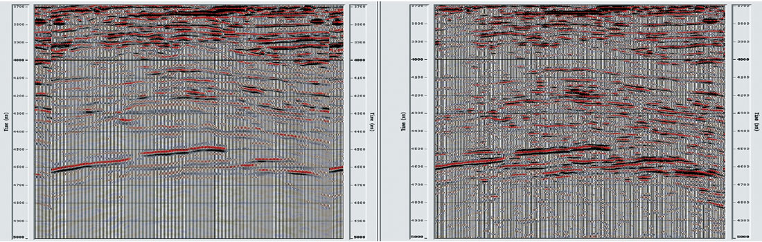
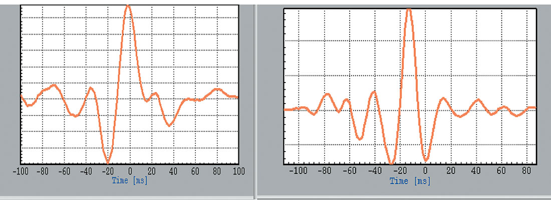
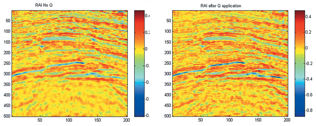
In figure 1 we present near angle stack before and after applying time-space varying Q filter on the data. In figure 2 we present the wavelet extracted using a well log and the seismic data before and after Q compensation. As expected, the wavelet after Q compensation has higher frequencies and is closer to zero phase. Note also that the wavelet is slightly noisier as can be seen from its side-lobes. In figure 3 we present relative acoustic impedance derived from the data presented in figure 1 using AVA inversion technique (see reference for more details). Note that there are differences associated with the two panels, and specifically, the low impedance zones are more delineated after applying timespace varying Q. Note that interpretation of the low acoustic impedance associated with the example bellow may result different reservoir properties estimates. Addressing potential attenuation affects on the seismic signal is part of the interpretational risk associated with seismic data processing flow, as discussed earlier.

Ran Bachrach

Question 2 — Answer 1

For such a general question, one can provide a general answer: we understand that thin layering above the target can cause transmission and interference effects that distort amplitude-versus-offset (angle) variations of reflections from target interval.

Yet, the distortion pattern and magnitude depend very much on peculiarities of the thin layer stack structure and diversity of the constituting layers’ properties. Depending on these particulars, it may or may not be possible to decrease the unwanted effects by either pre-processing or by specific interpretation measures.

First, a few general remarks about thin layering are in order. The AVO fundamentals were introduced about two and a half decades ago by considering a sole reflector as a boundary between two halfspaces. The implications of thin layers for AVO studies came into focus a bit more than a decade ago. Since then, trying to come closer to solving the problem of thin layer AVO, seismologists invented a series of remedies for thin layering effects removal – either in the form of AVO intercept and gradient corrections, or by filtering off the thin layering effects from the input data (Bakke and Ursin, 1998; Balz et al., 2000; Castoro et al., 2001; Dong, 1999; Gibson, 2005; Swan, 1997, 2002; Wapenaar et al., 1999; Widmaier et al., 1996). Some such remedies take care of reflection effects from fine layering within the target interval, and others are intended for suppression of propagation effects in the finely layered overburden.

However, in our opinion, it is difficult to say that our industry has a non-contradictory AVO technology that can guarantee elimination of the unwanted effects of fine layering.

On one hand, all commercially available AVO packages support creation of synthetics from blocked sonic log data. One is free to apply as fine blocking as one likes, so the procedure seemingly accounts for thin layer structure of the reservoir and overlaying formations automatically. Hence, we can count on reliable synthetics – within the limits of validity of the convolution or downward extrapolation model we use to represent seismic trace. Yet, it is not clear how this fundamental tool for studying fluid/lithology substitution effects may comply with the tools for suppressing thin layering effects.

On the other hand, during interpretation, we put aside all our considerations on fine layering and boldly ascribe the imaged anomalies to one of 3 (or 4) classes, introduced by Rutherford and Williams, 1989 (or Castagna and Swan, 1997) to describe the effect of a sole boundary between sand and overlying shale. (Recently, Young & LoPiccolo, 2003, proposed a 10 type anomaly classification, but this approach has not yet become a tool for everyday use with reliably reproducible results).

One can ask – what’s wrong with ascribing a certain class of (sole boundary) AVO anomaly to an imaged object as soon as one did one’s best to account for thin layering? It is a good question – meaning it is “hard to answer”. It is hard to answer indeed because, first of all, the remedies for thin layering effects mentioned above have not yet become a common practice. Second, each one of these remedies is designed in the framework of a certain theoretical model, and the remedy efficiency is confirmed on synthetic examples generated using the same model. Note: in all these theoretical examples, the modeled NMOed zero phase events generated from finely layered stacks and distorted by NMO stretch and differential NMO effects look nearly perfectly horizontal on the common image gathers at their arrival times – never mind the fine layering. There is every reason to believe that the remedies proposed will perform well on real data gathers, as well as on synthetic ones, provided the target events on these gathers are horizontal indeed. Unfortunately, in real data, much too often we come across migrated gathers where target NMOed events remain systematically and essentially nonhorizontal – though we are sure that this effect has nothing to do with wrong NMO velocity. Nothing of real value can be expected from applying AVO to such data. So what is the reason for the lineup distortions? In our experience, sometimes these distortions are successfully modeled by routine creation of synthetic gathers for blocked velocity and density logs, sometimes not. That is, sometimes our modeling tools confirm the fine layering nature of these distortions, and sometimes not – because either our modeling tools are inadequate, or there is some other - unknown - reason for the distortions besides fine layering. In any case, there certainly are formations where one cannot rely on today’s AVO techniques, with or without the corrections for fine layering reflection and propagation effects.

So we come back to where we started. All the above is said for a sole purpose to show that actually, we do not understand quite well which remedy we should use to guarantee effective accounting for fine layering – except, probably, creation of correct synthetics at every common image gather and performing global inversion to ensure satisfactory agreement between synthetics and field data by step by step adjustment of thin layer structure and lithology and saturation until the current synthetics agree with real data. Clearly, this global inversion approach requiring extraordinary computing resources can be effective only where there is a dense network of wells to calibrate AVO anomalies. In short, further theoretical and experimental work is needed to create AVO preprocessing and/or AVO inversion tools capable of solving exploration problems in the most complex cases of finely layered target and overburden strata.

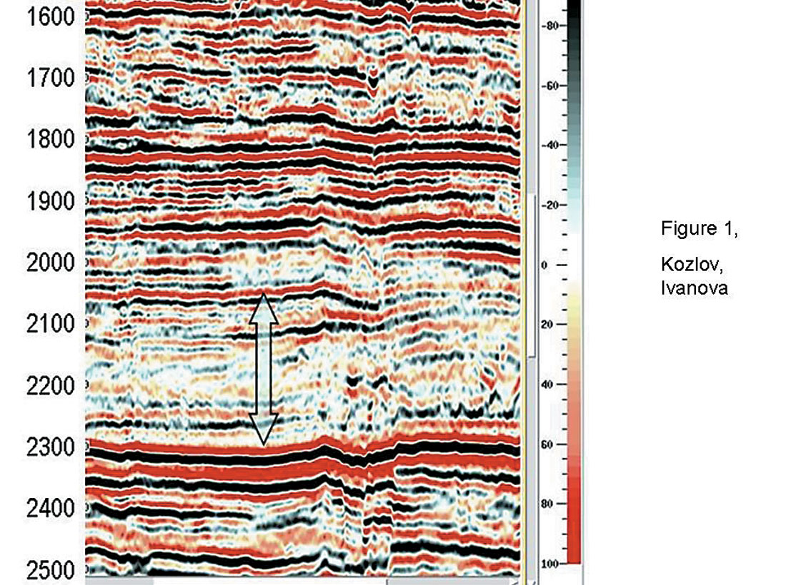
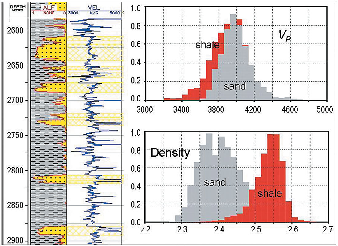
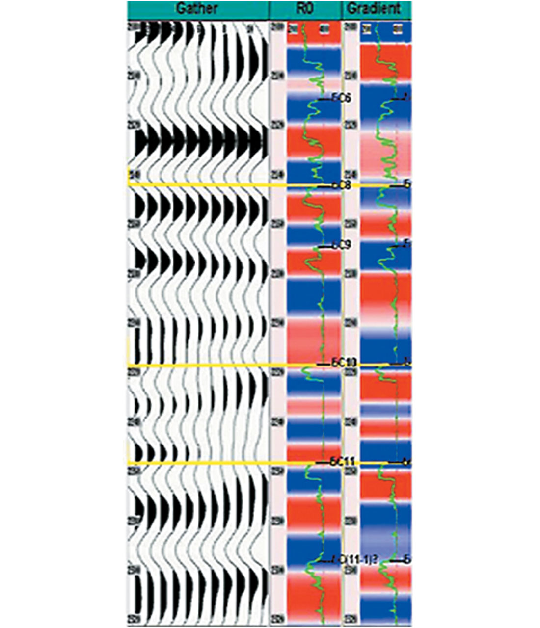
Now we want to illustrate this notion by a real data related to a Lower Cretaceous sandshale fine layering fan delta sequence of distinct sigmoidal structure, West Siberia, Figure 1. As compared to enclosing shale, the target sand layers have nearly the same P-wave velocity and essentially lower density, Figure 2. The reflectivity is laterally unstable, so no continuous seismic horizons can be traced within the formation, and at the migrated common image gathers, events in the vicinity of target layers are essentially non-horizontal on both the real and synthetic traces (the latter are calculated using good quality sonic and density logs from several tens of wells), Figures 3. On the ground of fluid/lithology substitution studies and well log evidence, it was concluded that variations of target layers’ porosity, saturation, and thickness produce effect on AVO attributes that cannot be distinguished from each other without auxiliary information. Indeed, AVO analysis carried out with all due preprocessing procedures yielded attribute cubes that took exhaustive interpretational efforts – which are outside the scope of this short text.

Note: the fine layering issues affecting AVO negatively are related to local peculiarities of the target interval. The overburden has also essentially fine-layered structure, but it is stable laterally, so its amplitude and phase offset-dependent effects on the target interval are negligible as compared to problems caused by the structural peculiarities of the target itself. In turn, due to low reflectivity within the target interval here, it does not affect the AVO efficiency in productive Jurassic formation underlying the interval we consider as the target. Let us hope that difficulties encountered at this particular field are local not only in space, but in time as well AVO is a rather mature technique, but its progress continues, and there is every reason to count on further achievements – first of all, in the line of a wider use of synthetic gathers created with a closer integration of petrophysical and structural data, than we can afford now.

Evgenii Kozlov and Natalya Ivanova,
Paradigm Geophysical,
Moscow

Question 2, Answer 2

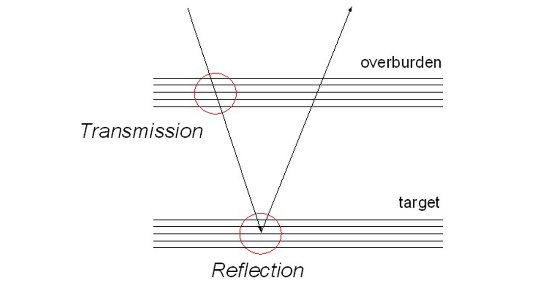
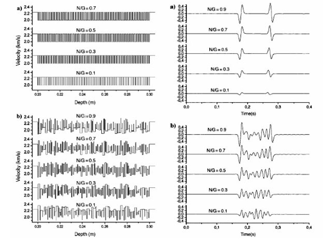
This is a very complicated and important question which is still a research issue. Most of the work within this area has been focused on elastic case only. We have to consider both transmission and reflection effects (see Figure 1). Both amplitude and phase velocities are frequency dependent. First of all we would like to mention the remarkable O’Doherty-Anstey (1971) formula for transmission amplitudes (low frequency limit). There are two main issues: layering and contrast (relative difference in elastic properties). The weak-contrast approximation of this problem can be found in Widmaier et al. (1996), the random medium approximation (still weak-contrast) can be found in Shapiro and Hubral (1999). Both these publications are easy and straightforward to implement and test for practical use. An alternative approach is given in Ursin and Stovas (2002, 2003). An example on how to use the latter approach for net-to-gross estimation for a turbidite reservoir is presented in Stovas, Landrø and Avseth, 2006. For quasi-vertical propagation with no limitation on contrast and layering, the amplitude and phase effects are discussed in Stovas and Arntsen (2006a). They also proposed an approximation for the phase velocity in a finely layered medium (2006b). These equations are straightforward to implement and test. The fundamental case (periodic medium) results in analytic expressions for transmission response for vertically propagating waves (Hovem, 1995; Stovas and Ursin, 2005). It is shown that between time-average and effective medium (Backus, 1962) there is a transition zone (attenuating bands in frequency domain) which corresponds to seismic resonance. The effective medium parameters: amplitude and phase velocity and the width of the transition zone are controlled by the contrast in elastic properties (reflection coefficient for vertically propagating waves). Perturbed thin-layer media are discussed and tested in Stovas, Landrø and Avseth, 2006, a comparison between non-perturbed and perturbed fine-layer models is shown in Figure 2. We notice a significant difference in the reflectivity pattern between the top and base reflections. However, the seismic amplitude changes for the top and base interfaces are small, but not negligible.

There are also some very interesting experimental papers by Marion and Coudin (1992) and Marion et al. (1994) demonstrating thin layer effects measured at ultrasonic frequencies.

For non-vertical propagation in arbitrary finely layered medium, the transmission amplitude and phase are extremely complicated due to the contribution of converted waves. Although, the quasi-vertical approximations for the reflection response, taking into account converted waves, were considered in Stovas et al (2004, 2006). Different cases for the contrast in elastic properties were considered in Stovas et al. (2006).

Foldstad and Schoenberg (1992) showed that a stack of thin layers can be approximated by an effective anisotropic layer. If a well log is available (giving information on velocities and densities within the thin layer zone) this approach can be used to estimate AVO-correction terms. Again, this is straightforward to implement, as soon as the anisotropic parameters have been determined. Another calibration option might be to compare modelled AVO-responses for one interface above the thin layer zone with another interface below this zone. If the average Q-Value for the zone between the two interfaces is known, it should be possible to compute an AVO-calibration curve based on simple comparison between the deviations between the observed and modelled AVO-curves (after correcting for the Q-absorption effect).

Martin Landrø, Alexey Stovas
Department of Petroleum Engineering and Applied Geophysics
Norwegian University of Science and Technology
Trondheim, Norway