Fractures in subsurface formations influence production and reserves of oil and gas, besides helping us understand the migration of these hydrocarbons. Knowledge of fracture distribution is therefore important and consequently there is a lot of interest in seismic characterization of fractures in subsurface formations. We feature the following question on fractures in the ‘Expert Answers’ column in this issue and hope that the readers will find the answers useful.
The ‘experts’ answering the question are Enru Liu (British Geological Survey, UK) and Chris Thompson (4C Exploration Ltd., California, USA).
The order of the responses given below is the order in which we received them. We thank the experts for sending in their responses.
Question
Fracture characterization of reservoirs is very important as it can have a profound effect on their productivity. So for improved reservoir management seismic fracture characterization is attempted.
In your expert opinion, what are the methods available for such a characterization for both conventional 3D P-wave data as well as multi-component data? What are the differences in characterizing clastic and carbonate reservoirs? Briefly explain the basic principles employed by the different methods and illustrate with examples.
Answer 1
Before I attempt to answer these questions, let me start with the definition of what we mean by seismic characterization of fractures. Seismic fracture characterisation normally refers to the interpretations of measured directional variations of seismic attributes (e.g. travel-times, velocity, amplitude, attenuation, etc.) in terms of fracture distribution (orientation, density, fluid properties, etc). This is known as seismic anisotropy that is defined as “Variation of seismic velocity depending on the direction in which it is measured” ( according to Sheriff’s Encyclopaedia). I was once told that “All reservoirs should be considered as fractured unless and until proven otherwise”, and thus seismic anisotropy should be regarded as very common.
Natural fractures in hydrocarbon reservoirs can be very complex as the geometry and distributions of fractures and fracture networks depend critically on the state of stress (past and present) as well as many other geological factors. We have to make some simple assumptions about fractured reservoirs, and typically we assume that most reservoirs contain one or more sets of nearly vertical fractures. If there is one set of vertically aligned fractures, the resultant medium will show Transverse Isotropy with a Horizontal axis of symmetry or HTI. For a medium with two orthogonal sets of vertical fractures, we have an orthorhombic symmetry (for details, see two papers on the terminology by S. Crampin in Geophysical Prospecting, 1989 and D. Winterstein in Geophysics 1990). Most of the time, when we talk about fractures, we assume one set of (near-) vertical open fractures in reservoirs (although other models, such as multi-fracture sets, or fractures in a VTI matrix are also sometimes used).
What fracture parameters can we extract from seismic data?
A detailed description of fracture patterns will require many parameters, and it is certainly not practical to describe each individual fracture in a fracture network. However, what we are interested in are the parameters controlling the elastic response and eventually hydraulic or flow response. Two parameters that we can reliably extract from seismic data are fracture orientations and density, and to a lesser degree fluid properties (fluid types). There are many successful examples, see for examples, papers published by Heloise Lynn et al. in Geophysics. Recently, we have argued that fracture size may also be estimated through measurements of frequency-dependent anisotropy (see E. Liu et al., July 2003, The Leading Edge; and S. Maultzsch, et al. July 2003, First Break). Other fracture parameters, such as spacing, aperture, etc will be difficult, if not impossible, to estimate.
Note that the physics behind seismic characterisation of fractures is based on various equivalent medium representations of fractures (see, for examples, E. Liu et al., J. Geophys. Res. 2000 and M. King, Geophysics 2005 for recent reviews). Perhaps the mostly common model has been the one developed by John A. Hudson of University of Cambridge (and various extensions afterwards). A model proposed by my colleague Mark Chapman (Geophysical Prospecting 2002) addresses fractures in porous media and it has two scales, i.e., microscopic pore/cracks and meso-scopic aligned fractures. The model predicts frequency-dependent anisotropy and forms the basis of fracture size estimation from seismic anisotropy.
A common parameter in almost all theories that describe the seismic wave propagation in fractured rock, which is related to the magnitude or degree of anisotropy, is the fracture density ε. It is defined as the number density γ of cracks multiplied by the cube of the crack radius α: ε = γ α3 (where γ=N / V, N is the number of fracture, V is the volume). This definition of fracture density has no specific basis, and is introduced purely for mathematical convenience. This definition is not the same as the definition used in engineering literature. Engineers define fracture density as the number of fractures per length. It is not easy to reconcile the two definitions as the geophysicists’ definition involves two scales (fracture radius/length and volume), but engineers’ definition has only one scale (length in which the number of fractures is measured). One possible way to reconcile the two definitions may be as follows: If we assume a standard crack geometry with N=250 aligned vertical fractures of diameter D=2a=0.2m (a is crack radius) and separation perpendicular to the fractures S=1/C=0.1m in volume V=1m3 (C is the number of fractures per metre), the fracture density is ε =N a3/ V= 250* 0.13/1=0.25. If instead we consider a cube with side D, then ε =C D a3/(2D)3=C D4/8D3=10*0.2/8=0.25.
What are the methods available for seismic fracture characterisation?
Below I shall discuss briefly the principles of estimating fracture orientations and density from various seismic methods.
Multi-component S-waves
From the middle 1980s until the middle 1990s, technology based on multi-component shear-waves was popular. The idea is that when a shear-wave enters an anisotropic (fractured) medium, the shear-wave will split into two: one travels faster, the S1 or fast S-wave and another one travels slower, the S2 or slow S-wave. This is known as shear-wave splitting or birefringence. The polarization (or vibration direction) of the fast S-wave is in the fracture plane (strike) for HTI media, while the time-difference or time-lag between S1 and S2 is roughly proportional to the fracture density. In the early days, S-wave polarization was measured manually from histograms or polarization diagrams (still used for earthquake data). Later, various techniques were developed to extract shear-wave polarization and time-delays between the two-split S-waves, including the famous Alford rotation (Alford, 1986 SEG Expanded Abstract) and various layering-stripping techniques. Note that because of the nature of S-waves and the complication of near-surface effects (e.g. S-wave window), it is better to analyse shear-wave data for near vertical raypaths.
Shear-wave acquisitions have gradually declined since the middle 1990s as shear-wave data were considered to be too expensive to acquire and required large data storage (for 3- components). In particular, shear-wave data typically have low frequency contents and data quality is not as good as P-waves. However, we at the Edinburgh Anisotropy Project and Tom Davis’s Reservoir Characterization Project in Colorado School of Mines are still very active in acquiring and analyzing multicomponent shear-wave data.
3D P-waves
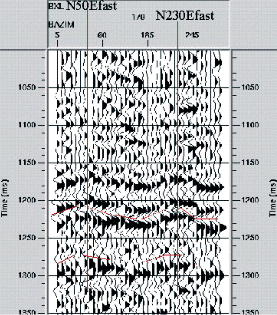
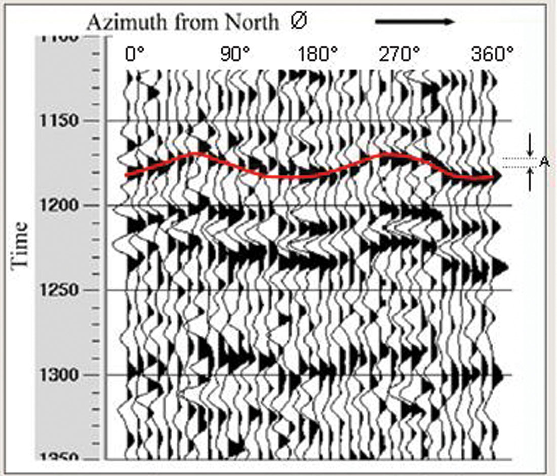
Over the past ten years, there has been a steady increase in using 3D seismic data to characterize fractures. If we assume the fracture population consists of predominantly one major orientation, we expect that waves travel faster along fractures than normal to the fractures. As a result, the azimuthal variations of P-wave attributes, such as travel-time, NMO velocity, reflected wave amplitudes, impedance, frequency, attenuation, etc. can all be approximately described by an ellipse. Afield example provided by Heloise Lynn in Figure 1 demonstrates clearly that azimuthal variations of P-wave travel-time (and amplitude) are sinusoidal functions. One axis of this ellipse indicates the fracture orientation, and the ratio of two axes of this ellipse is proportional to the fracture density or intensity of the rock concerned. The axis of minimum travel-time (short axis) or maximum NMO velocity (long axis) is interpreted as the fracture orientation. For amplitudes, it is a little bit more complicated (see below for explanation). As we know, at least three data points are required to define an ellipse in azimuthal planes (i.e. two axes plus the orientation). In practice, we do not normally fit ellipses, but rather fit a sinusoidal variation to P-wave attributes. There are many attributes that can be measured. At EAP, we prefer to utilize as many attributes as possible to perform multi-attribute azimuthal analyses (the technique is known as AVD – attributes versus direction, where “direction” includes both offsets and azimuths). Note that P-wave azimuthal variations increase with offset, and so typically we require the offset-depth ratio to be larger than one (in contrast to S-waves).
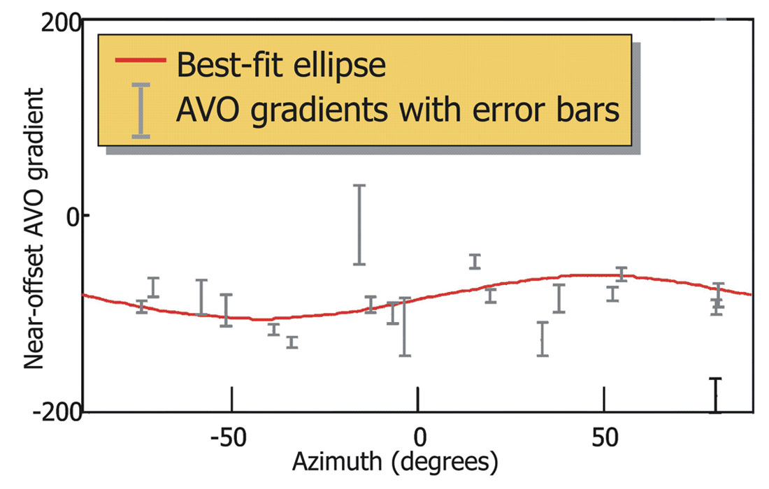
Two methods are often employed to extract the fracture information from P-waves: full-azimuth surface fitting and narrow-azimuth stacking. The first method fits an elliptical surface to data from all available azimuths and offsets by a least-square fitting technique. The second method divides the data into a number of narrow-azimuth volumes and the data in each azimuth bin are stacked. For example, 12 azimuths with a 30° azimuthal bin or 24 azimuths with a 15° azimuth bin can be chosen depending on the resolution required. Corresponding to these two methods, there are mainly five seismic attributes which may be used to extract the fracture information, including NMO velocity, reflected-wave travel-times, interval travel-times, reflected wave amplitude, and AVO gradient. The surface fitting method is applicable to the amplitude and travel-time attributes, whilst the narrow-azimuth stacking method is applicable to the velocity and AVO gradient attributes. An example provided by Steve Hall is given in Figure 2, which fits observed azimuthal variations of AVO gradient. Figure 2, which fits observed azimuthal variations of AVO gradient. A detailed analysis of a land 3D P-wave data is given in Li et al. (The Leading Edge, 2003 July issue).
Some notes on P-wave azimuthal AVO analysis.
Analytic P-wave AVO equations in fractured media have been derived by Rüger in his award-wining thesis/book (published by SEG as a monograph). In general, we can write PP-wave reflectivity across an anisotropic/ anisotropic boundary as a Taylor series expansion around (θ is the P-wave incident angle and ϕ is azimuthal angle measured from fracture normal direction):
RPP (θ,ϕ) = A+B (θ,ϕ)sin2(θ)+C(θ,ϕ)sin4(θ),
where coefficients A, B and C are PP-wave AVO attributes. As in isotropic media, A is called the AVO intercept and does not depend on the incident angle θ and azimuth angle f, B is the AVO gradient and C is the AVO curvature. The AVO gradient B (and AVO curvature C as well) varies with azimuth as
B(ϕ) =b0+b1 cos2(ϕ – ϕ0)+b2cos4(ϕ – ϕ0)
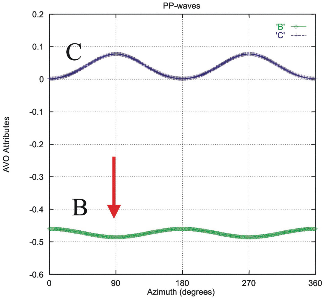
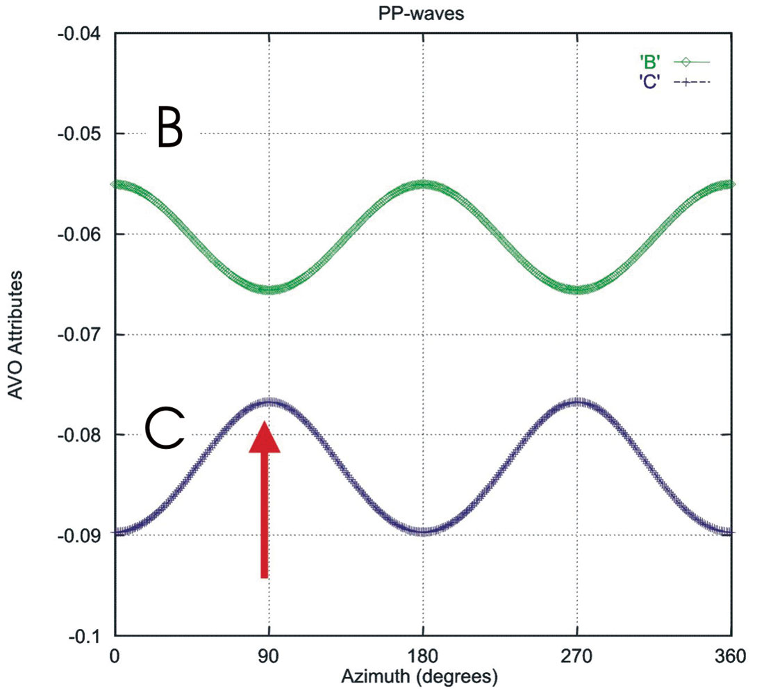
ϕ0 is fracture orientation. So we can fit the AVO gradient to a cos2ϕ function from which we can derive fracture orientation (see Figure 2). Whether the trough or peak of AVO gradient is fracture orientation depends on types of AVO. Figure 3 shows the variations of PP-wave AVO attributes B and C with azimuth for a Class I AVO model: for a shale/sand boundary (Vp, Vs and density for shale are 3.3km/s,1.7km/s, 2.35g/cm3 and for sand 4.2km/s, 2.7km/s, 2.49g/cm3). Similarly, Figure 4 shows the variations of PP-wave attributes B and C with azimuth for the Class III AVO model: for a shale/sand boundary (Vp, Vs and density for shale are 2.73km/s, 1.24km/s, 2.35g/cm3 and for sand 2.02km/s, 1.23km/s, 2.13g/cm3). These figures were calculated using the exact solutions through numerical calculations and then we fit the results using the above equations. From these figures, we observe that both B and C follow a variation. We also find that their variations are at the same order of magnitude for both classes of AVO models and the magnitudes are related to the fracture density, i.e. the higher the fracture density, the larger the azimuthal variations will be. In Figure 3, fracture directions are coincident with the peak in the variations of B (for class I type AVO) and in Figure 4, fracture orientation is coincident with the trough in the variation of B (for class III AVO). My colleagues Mark Chapman, Xiang-Yang Li and I have recently shown the effects of attenuation of PP-waves, and we argue that PP-wave amplitudes can vary as a function of frequency, and this can be related to the reservoir fluids (see Chapman et al., Nov 2005, The Leading Edge; and our 2004 SEG Expanded Abstract).
Finally, mention must be made of the technique advocated by Mark Willis and his colleagues in MIT. They propose to measure azimuthal variation of seismic scattering. The concept is simple: along fracture strikes, seismic waves suffer less scattering, while in the direction normal to fractures, seismic waves suffer most scattering (attenuation). As we move from parallel to normal directions, we expect a systematic increase in scattering. Willis et al. have applied their technique to synthetic and Emilio field data (see their 2004 SEG and EAGE abstracts).
PS or C-waves
PS-waves seen in OBC data or from land seismic surveys are essentially S-waves, and therefore most techniques developed to extract fracture information from pure S-wave data can also be applied to PS converted or C-wave data. Examples are various rotation algorithms, converted-wave splitting analysis, etc. Jim Gaiser of WesternGeco has proposed to use orthogonal lines of PS-wave data to form a 2 by 2 matrix and then to perform Alford-type rotation. Robert Garotta (CGG), Steve Horne (WesternGeco) and their colleagues propose to find directions of linearity or minima in the ratio of transverse/radial components based on the fact that P-waves will only convert to pure SV waves (in the radial component defined as from source to receiver) when source-receiver lines are parallel to fracture strike or fracture normals. Techniques have also been developed to look for polarity reversals in transverse components, based on the fact that PS-waves (P to SH conversion) recorded on transverse components will show a 90° polarity reversal across fracture strikes. Note that because of the variations of PS-wave reflection coefficients across a boundary, optimal offsets should be around the middle range, i.e. the offset/depth ratio around one.
What are the differences in characterizing clastic and carbonate reservoirs?
This is a difficult question to answer, but I believe in terms of purely the technology to extract fracture information from seismic data, there are essentially little difference between clastic and carbonate reservoirs. In clastic reservoirs, fluid flows are not necessarily controlled by fractures, and therefore the estimation of fracture orientations is a less important issue. However, in carbonates, fluid flows are thought to be entirely controlled by open and connected fractures, and thus characterisation of fractures in carbonates becomes more important. However, carbonates are very complex, and the scales of heterogeneity distributions can span up to six orders of magnitude. The geometry of fractures in carbonates can also be complex, and so is the fluid substitution problem; these make the (equivalent-medium) modelling of seismic wave propagation in fractured carbonates very hard. I believe the multi-scale fracture models that we have developed in Edinburgh and the estimation of fracture size distributions using the frequency-dependent anisotropy concept will advance our understanding of seismic behaviour in fractured carbonates, and new technology will emerge along this line.
Acknowledgements: I thank Heloise Lynn and Steve Hall for allowing me to use their figures in this note.
Enru Liu
British Geological Survey, UK
Answer 2
To address a technical question it never hurts to go back to the basic science, the physics. This is particularly true for such as fracture characterization. For most specialized areas of seismology, the science is well understood, and the complicated parts usually are in the application and implementation. Interestingly enough, as a scientific community we don’t fully understand what happens to seismic waves as they impinge upon a discontinuity such as a fracture. However, in the past decade of so, significant progress has been made in our theoretical understanding of the seismology of fractures, and on an empirical level, we have made enough observations, both in the laboratory and in real data, to be able to categorize pretty well how seismic waves behave in a fractured medium. For instance we know that the shape and contacts of the surfaces of the fractures are important, as are the number of fracture sets and their orientation. So we don’t yet have the final answers in this subject, but we clearly know enough about it to use it as an exploration and development tool.
It turns out that seismic waves are slowed and attenuated when they cross a fracture boundary. The fractures make the rock more compressible and compliant in the direction normal to the fractures. The effect appears to be more pronounced if the fracture is gas-filled or filled with a compressible fluid. A side product of attenuation is that the effect is also frequency-dependent, with higher frequencies preferentially attenuated across the fracture. On the microscopic-scale, current thinking is that the fractures weaken the rock for both P and S waves, absorbing the higher frequencies as the fluids ‘slosh about’ in the fracture pore space.
If the fractures are organized in a given direction, this leads to an asymmetry to the wave front as it passes through the fractured volume. The simplest case is where the fractures are oriented vertically, with a single (compass) direction to the fracture strikes. This is the socalled “horizontal transverse isotropy” or HTI geometry. Of course, fractures can come in multiple sets with non-vertical orientations, and to describe seismic waves in those cases the mathematics can get ugly in a hurry. Fortunate for us, cases of near-vertical oriented fractures are not that uncommon geologically, and have a first-order effect on reservoir fluid flow. Recent research to describe the more complex cases is advancing steadily; for the pragmatists amongst us, techniques that are based on a single vertical fracture set now are mature enough for wide-spread use.
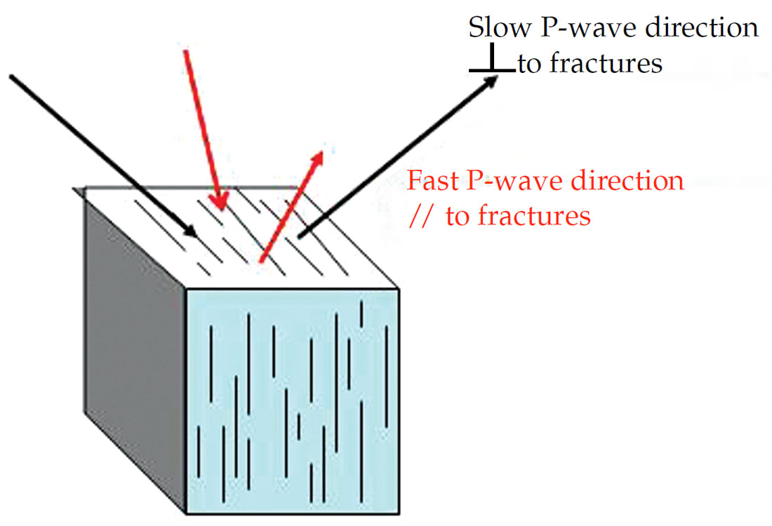
For a compressional (“P”) wave passing through a vertically fractured volume, it’s the horizontal component of the P-wave that passes perpendicular to the fractures that is slowed and attenuated, while the vertical component has particle motion parallel to the cracks and is relatively unaffected (see Figure 1a). So for surface seismic geometries, the slowing and attenuation have their strongest effect on the far offsets. The effect on the far offsets depends on the compass direction of the P-wave. If the fractures strike North-South, then the East-West directions will be slowed and attenuated. We can use this quality of P-wave to help characterize fractured reservoirs.
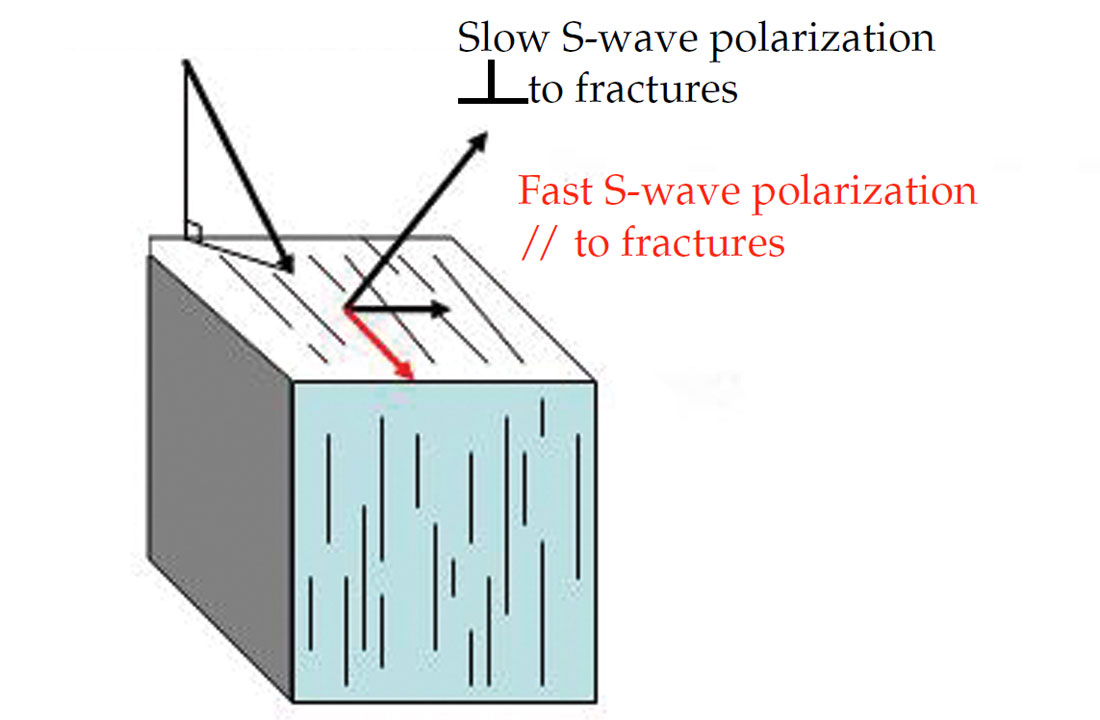
For shear waves (“S”) waves passing through a vertically fractured volume, particle motion is perpendicular to the direction of propagation, so the vertical component of the S-wave is most strongly affected. We like to describe the S-wave field as then polarized into ‘fast’ and ‘slow’ directions. For the same North-South striking fractures, the North-South polarization direction will be ‘fast’ and the East-West polarization will be ‘slow’ and attenuated (see Figure 1b). Again, we can use this azimuthal anisotropy (also known as ‘shear-wave splitting’ and ‘shear-wave birefringence’) to characterize the fractured rocks through which the shear wave passed.
So based on our admittedly incomplete understanding of the physics, but emboldened by empirical success, we can characterize simple fractured reservoirs using the slowing and attenuation of both P and S waves.
Practical application. The most obvious way to use this behaviour is through analysis of P-waves. If you examine the far-offsets of a surface seismic P-wave dataset, you may find that the arrival times for a given reflection fluctuate based on the direction of travel (see Fig 2). Assuming a single orientation for vertical fractures, we can fit a ACos2Ø curve to the travel times from different azimuths, where Ø is the azimuth of fracture orientation and ‘A’, the amplitude of the azimuthal variations, is a measure of the relative fracture density.
A number of the service companies can run these analyses to derive fracture orientation and fracture density from the arrival times of surface seismic reflections. One implementation of the processing can be to ‘correct’ for the azimuthal variation in arrival time, which can make a huge improvement to the S:N of both the stack of all the azimuths, and pre-stack AVO analysis. An underlying assumption in the approach is that the observed azimuthal variations are caused by the reservoir interval of interest. One needs to check that azimuthal variations are not present in the overburden, and if they are, to ‘layer-strip’ away the overburden effect to focus on the reservoir effect.
We also tend to assume only one vertical fracture orientation. If the fractures are non-vertical, or if there are multiple fracture sets, then a more sophisticated forward model will be required to interpret the data.
Unfortunately, most of our existing land and marine 3D seismic datasets are not well suited to these analyses, typically because of limited azimuth sampling of the crucial long offsets. For standard marine streamer data the geometry has very narrow azimuths and is entirely unsuitable for fracture characterization (both the source and receivers are pretty much directly behind the boat). For marine fracture investigations either multiple streamer passes are required, or a seabed survey with either a square patch of nodes and shots, or an OBC cable survey with shot lines orthogonal to the receiver lines is best. On shore, roughly square receiver patches and roughly square source patterns can give good sampling in both azimuth and offset. These geometries can be slightly more expensive to record, and unless the azimuthal effects are taken into account in processing the stack data quality can be degraded. Most vintage on- shore 3D surveys are still somewhat narrow azimuth for good P-wave fracture analysis.
Not only are the P- travel times delayed in a fractured medium, but the amplitude is attenuated and the phase rotated. For wide-azimuth, long- offset data, these characteristics can also be used for fracture characterization, although the technique is still rather new. Researchers fro m Edinburgh Anisotropy Project and elsewhere are studying this approach (e.g. Chapman et al, The influence of abnormally high reservoir attenuation on the AVO signature, TLE, Nov 2005).
As described above, shear velocities are also anisotropic in the presence of fractures. The most common way to use this for fractured reservoir characterization is to look for azimuthally varying P-wave AVO (sometimes referred to as ‘AVOAz’), since the offset behaviour is strongly influenced by the anisotropic shear velocity (as well as the P velocity). Provided that the surface seismic data are well-sampled in azimuth and offset, this approach can be effective and relatively inexpensive. Figure 3 shows an example from a Central Texas shale reservoir where AVOAz analysis seems to be identifying the azimuth and the relative fracture density of a dominant fracture set.
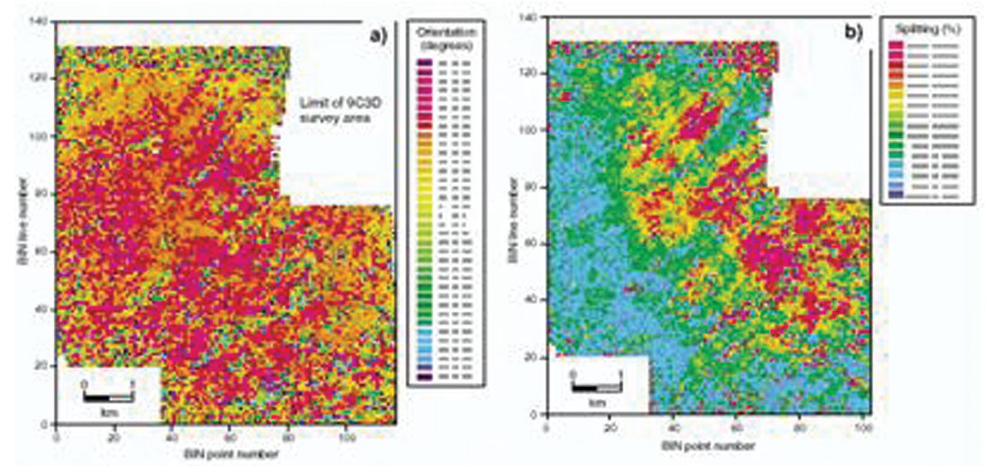
One can directly measure S-wave anisotropy from fractured reservoirs using 9C data (shear source & receiver) or 3C data (P-Source used to generate converted shear waves which are then recorded in 3C receivers). One of the earliest and best examples of this is from onshore Oman, where the direction and density of known fractures of the carbonate reservoir was characterized by using shear wave splitting from a 9C survey (see Figure 4 from Hitchings & Potters, TLE 2000).
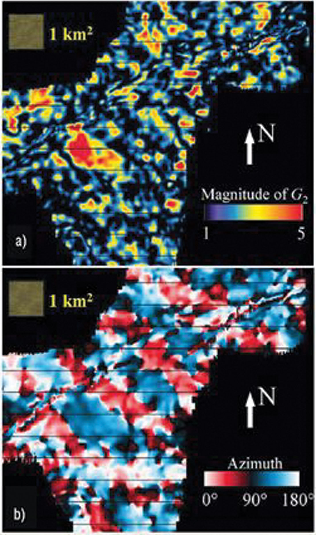
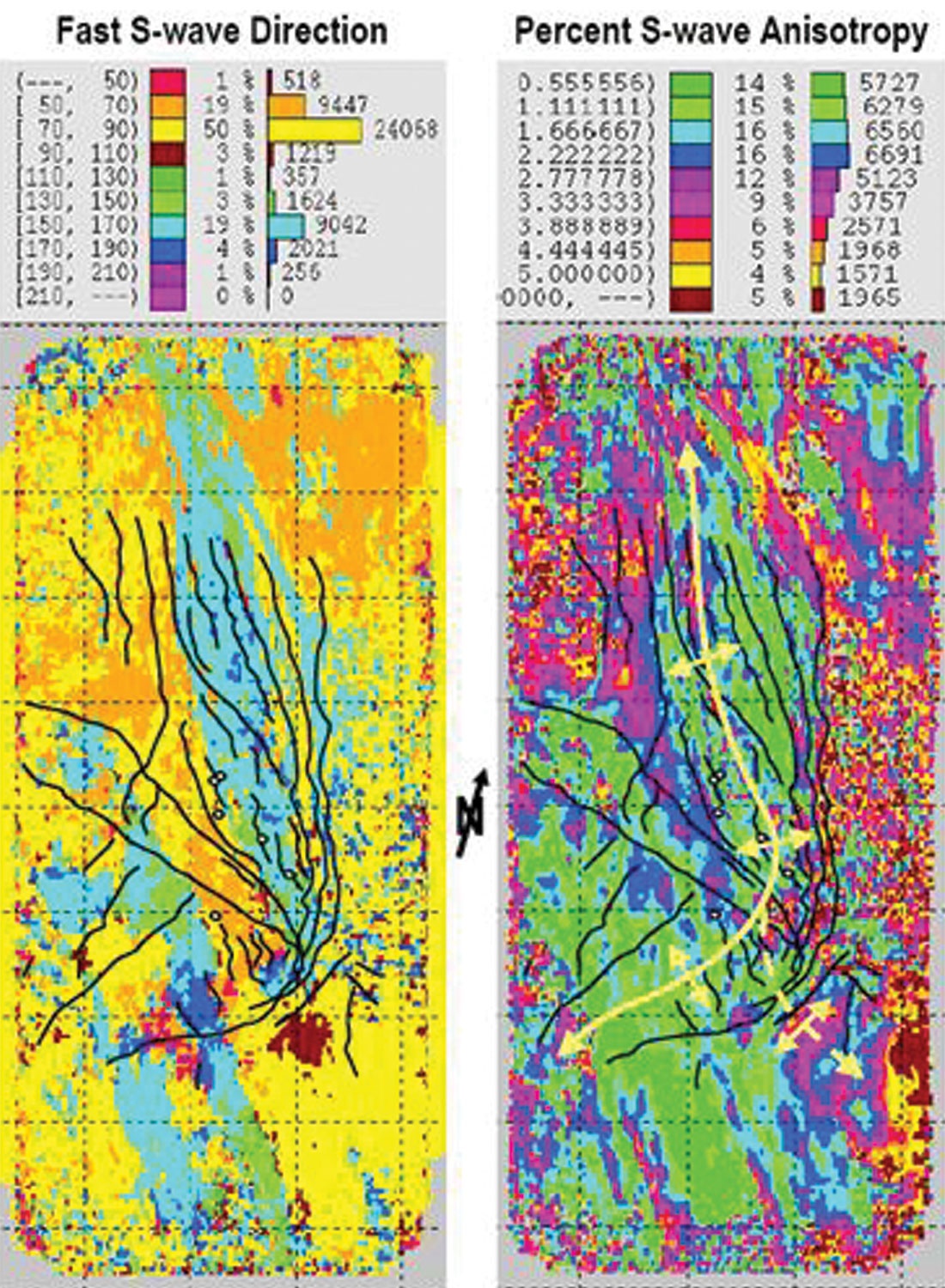
Similar results can be generated offshore using converted shear waves from a 4C survey. Figure 5 illustrates the changing fracture orientation and relative fracture density of the Emilio Field, Adriatic Sea which nicely agrees with known fractures from well control. Again, the seismic fracture characterization reveals the fault-bounded compartments of the field flow units. Areas of maximum anisotropy seem to be along the folded leading edge of the thrusted carbonate hanging wall, in places where tectonic stresses are likely to be highest, and fractures are likely most dense. The authors later successfully extended this work to derive the non-vertical fracture axes over the field.
Implementation. These examples are not just isolated cases – the technology is mature enough for widespread use. Geoscientists who need to characterize fractured reservoirs should consider a number of possible approaches. Typically one of the most difficult tasks is pulling together the funding and management approval to do the seismic fracture characterization. Often the best approach is through a series of low-cost, low-commitment steps. First, understand the geology of the fractures – are they thought to be restricted to the reservoir interval, are they mostly aligned and vertical? Next, forward modeling with one of the service companies or academic groups can tell you about the size and nature of the seismic anomaly you should expect to see over the field. From there, if you have a suitable 3D seismic dataset with wide azimuths and offsets, you can check for azimuthal variations in reflection arrival time and AVO character. Azimuthal P-wave reprocessing would then be a relatively inexpensive means of fracture characterization. A similar analysis with 2D data of different azimuths can also yield compelling results.
If you don’t have a suitable 3D dataset, and the value of fracture characterization can be supported by the potential increase in production from the field, you may have to commit to the time and expense of new acquisition. One relatively low-commitment approach to this is to record a VSP first. Re-entering a borehole or using a newly drilled well may give you the opportunity to record additional well logs, such as a cross dipole sonic log and a walkaway or walk-around VSP. With the VSP results in hand, you should be able to justify or reject the expense of a full-azimuth P-wave, 3C, 4C or 9C 3D-survey.
Acknowledgements: The author would like to thank Greg Ball of Chevron Exploration Technology Company for insightful editing of this article.
Chris Thompson
4C. Exploration Ltd.
California USA


Share This Column