Expert Answers

Question

Fluid substitution essentially refers to prediction of seismic velocities in rocks saturated with one fluid from dry rocks or rocks saturated with another fluid. Gassmann’s equation has been frequently used for such prediction of effects of fluid saturation on seismic properties.

• What are the assumptions on which Gassman’s equation is based and how accurate are its predictions?
• Is Gassmann’s equation applicable to only particular lithologies, i.e. valid for certain types of sandstones and not valid for carbonates? How about its application to laminated shaly-sands or a fine-layered sand shale sequence?
• If the rocks are dry and anisotropic, is there a way to predict seismic velocity for fluid saturated anisotropic rocks?
• What are some of the other ways of addressing the problem of fluid substitution?

Answer 1

Fluid substitution refers to prediction of seismic velocities in rocks saturated with one fluid from dry rocks or rocks saturated with another fluid. Gassmann’s equation has been frequently used for such prediction of effects of fluid saturation on seismic properties.

Q: What are the assumptions on which Gassman’s equation is based and how accurate are its predictions?

Seismic fluid substitution modeling using Gassmann’s equation has become routine in the analysis and interpretation of seismic velocities and amplitudes. Fluid substitution is central to quantitatively understanding seismic attributes for hydrocarbon detection, analyzing 4D seismic, and even for understanding seismic signatures of lithology and porosity, since lithologic signatures usually have fluid effects superimposed. Gassmann’s equation is remarkably robust and general. When used under the appropriate conditions, it is usually as accurate as the measurements of saturation, velocity, and porosity that go into the equation. However, as with just about any quantitative tool in geophysics, petrophysics, or rock physics, “the devil is in the details.”

Gassmann derived his famous equation using a rigorous mechanical analysis. His theory assumes that a dry rock behaves as a porous linear elastic solid with well defined elastic bulk modulus (reciprocal of compressibility) and shear modulus. The pore fluid is assumed to interact with the solid only by applying pore pressure to the internal surfaces of the pore space. As compressive stress is applied to the external surfaces of the rock (for example, stress from a passing P wave), the frame elastically compresses; the compression squeezes the pore fluid, which induces an increment of pore pressure. This pore pressure resists the compression of the pore space, hence, stiffening the rock. Some specific assumptions of the theory:

1) Gassman theory assumes that the solid phase of the rock is elastic and homogenous. Strictly speaking, Gassmann theory applies only to monomineralic rocks – for example, pure quartz sandstones, or very clean limestones. In practice, rocks usually have mixed mineralogies. To get by, we usually cheat a little bit by estimating the average bulk modulus of the mineral mix, and then substitute this average into Gassmann’s equation. Normally, this assumption works well, although clay presents special problems. The elastic moduli of clay are very much smaller than those of quartz, feldspar, calcite, and dolomite, so that large amounts of clay can cause the average-mineral method to introduce errors. Furthermore, pore filling clay and structural clay impact the fluid effects differently, so that the best mineral-averaging scheme becomes lithology-dependent. Brown and Korringa published a generalization of Gassmann’s equation that allows for mixed mineralogy, although their theory requires an additional constant, which again is sensitive to the details of how the minerals are distributed at the microscopic scale. Hence, this constant is difficult to determine.

The good news is that at high porosities (> 20%), the Gassmann predictions are relatively insensitive to the details of the mineralogy; at smaller porosities, errors in mineral moduli become more problematic.

2) Gassmann theory assumes only pure saturations, for example, 100% water, 100% oil, or 100% gas, without mixtures. Reservoirs always have mixtures of fluids: oil and water, gas and water, or all three. To get around this, we estimate the average density and compressibility of the mixture of pore fluids and substitute these averages into Gassmann’s equation (another cheat). Unfortunately the proper way to estimate the effective compressibility of the fluid mix is not unique, but depends on the way in which the water, oil, and gas are distributed throughout the pore space. We have to consider whether the fluids are uniformly mixed at a fine scale, or whether the saturation is “patchy.” Choosing the appropriate fluid mixing rule is very important when there is free gas, but is relatively unimportant in oil-water systems.

3) Gassmann theory assumes isotropic rocks. The most common form of Gassmann’s equation assumes that the minerals making up the rock are isotropic (almost never true) and that the pore space and mineral distributions are statistically isotropic without a predominant alignment or fabric. (Actually, Gassmann also published an anisotropic version of his famous equation, although we seldom know enough about our rocks to use it.) In practice, the most common approach is to ignore rock and mineral anisotropy, although the practical consequences of this have not been well established.

4) Gassmann theory assumes perfect communication of the fluids in the pore space. When a passing wave squeezes on a rock, heterogeneities in the pore space lead to microscopic pore- pressure gradients and subsequent flow of the pore fluid. Gassmann’s theory assumes that the fluid can easily flow and relax these wave-induced pore pressure gradients during a seismic period. This assumption applies best to low viscosity pore fluids and to high porosity rocks with good pore space connectivity. Situations that can lead to trouble include very heavy oil, very high frequencies (as in laboratory ultrasonic measurements), high shale content, and low permeability.

Q: Is Gassmann’s equation applicable to only particular lithologies, i.e. valid for certain types of sandstones and not valid for carbonates? How about its application to laminated shaly-sands or a fine-layered sand shale sequence?

The answers to these questions lie in the assumptions that I have already mentioned. I have used Gassmann successfully in clean and dirty sandstones, limestones, and chalks. The presence of a lot of clay complicates the estimate of appropriate average mineral moduli that we need as an input into Gassmann’s equation. Also, clay inhibits the movement of fluids in the rock, which can lead to a breakdown in Gassmann’s assumption of easy fluid flow within the pore space. We cannot use Gassmann’s equation to compute fluid substitution in shale, but of course, we don’t usually need to worry about fluids changing in shale. Heavy oil (high viscosity) will also lead to violation of easy-flow assumption. Microporosity within clay or other grains leads to complications – one approach to dealing with this is to consider the microporosity to be part of the “mineral,” but then the elastic moduli of this microporous mineral is difficult to estimate.

Regardless of the rock type, I generally do not expect Gassmann’s equation to describe fluid effects at ultrasonic frequencies, where there is simply not enough time for the fluid to flow and equilibrate during the ultrasonic period. One mistake that I see too often is that people “test” Gassmann’s equation on ultrasonic laboratory measurements on dry and saturated rocks. When Gassmann’s equation does not explain these high frequency data, they conclude that Gassmann’s theory is wrong and should not be used in the field. This is nonsense. Lab and field situations are completely different when it comes to fluid substitution.

A few recent publications, as well as some of my own on-going research, indicate that special care must be taken when working with laminated shaly sands. Gassmann’s equation is still appropriate in the thin cleaner sand layers, but not in the low permeability shale layers. If the layering is finer than the sonic or seismic wavelength, then applying Gassmann’s equation brute force to the measured velocities will lead to an overprediction of the fluid sensitivity. However, if we “down-scale” the problem and only apply fluid substitution to the sand laminae, then we’ll be more accurate. The key here is to have some independent information that the laminae are present, what fraction is sand, and what are the porosity and elastic moduli of the sand.

Q: If the rocks are dry and anisotropic, is there a way to predict seismic velocity for fluid saturated anisotropic rocks?

Anisotropic fluid substitution equations have been published by Gassmann and later by Brown and Korringa. Both of these share the same assumptions of an isotropic mineral modulus and a well-connected pore space. The equations are simple to program and to use. However, they require knowledge of the complete elastic tensor of the rock, which we seldom know. For a transversely isotropic rock, we need 5 independent anisotropic elastic constants, and for an orthorhombic rock, we need 9 constants. In the field, the sonic log and density log will yield just one elastic constant, while adding a shear wave sonic will yield a second constant.

So what do we do? Most commonly, people just ignore the anisotropy and apply the usual isotropic Gassmann equation. Another approach (though rare) is to try to model the anisotropy, assuming something about the rock fabric, for example, aligned micro or macro fractures, aligned mineral grains, or lamination. If the rock is anisotropic because of finely-laminated sand and shale, then use the strategy that I mentioned in the previous question instead of applying one of the anisotropic fluid substitution equations.

I’m actually in the process of writing a paper on the difference between isotropic and anisotropic fluid substitution. I’ve found a few simplifying approximations that should help.

Q: What are some of the other ways of addressing the problem of fluid substitution?

The famous Biot theory also presents equations for how fluids impact the velocities of rocks. These attempt to describe the problem over the whole range of frequencies. In the limit of very low frequency, Biot’s equations reduce to the famous Gassmann equation. Quite a few years ago, we showed that Biot actually neglects some very important effects at very high frequencies. The short answer is that I almost never use Biot theory, and I don’t particularly recommend getting distracted by its mathematical elegance.

Another approach to fluid substitution is to use one of the penny-shaped crack models. The best-known are the ones of O’Connell and Budiansky, Kuster and Toksoz, and Berryman. The approach here is to model the pore space with a distribution of penny-shaped (ellipsoidal) cavities, evaluating the equations separately for dry cavities, oil-filled cavities, water-filled cavities, etc. It is extremely important to recognize that these models have perfectly disconnected pore space. Therefore, they give predictions very different from Gassmann. They have been relatively successful in describing fluid substitution under high-frequency laboratory conditions ( where Gassmann does not work well). We might also find that these work well for some tight rocks and very high viscosity oils, although I generally don’t recommend using these penny-shaped crack models unless you really know what you’re doing.

Finally, don’t use laboratory ultrasonic measurements on rocks with different fluids as an indication of the fluid effects in the field. This is generally just a bad approach, unless you have specific reason to think that the pore space is poorly connected in a way that will violate Gassmann’s assumptions. I’ve seen a few studies where lab data seemed to agree with field data in heavy oils, but be careful.

Let me summarize. Gassmann’s theory is remarkably accurate and robust. Most often, when disagreements are found between Gassmann and field measurements, it can be traced to mistakes – inappropriate mineral moduli, measurement errors in velocity, density, or porosity. When working with well logs, my experience has been that we are more likely to have problems from mud-filtrate invasion and measurement errors than with the theory itself.

Gary Mavko,
Stanford University

Answer 2

Response by Keith Katahara, Spinnaker Exploration Company, and Tad Smith, Veritas DGC Inc.

Basic Assumptions

Gassmann theory makes the following assumptions: 1) the rock is homogeneous and isotropic, 2) all the pores are interconnected (i.e., “effective” porosity), 3) the fluids are immiscible and homogeneously distributed, and 4) frequencies are sufficiently low enough for changes in pore-fluid pressure to equalize during sonic or seismic wave propagation (that is, the pore fluids are “relaxed”). It is important to note that Gassmann theory makes no assumptions about pore geometry. Thus, as long as these four key assumptions are valid, Gassmann theory should work well. However, it is well known that these assumptions often break down in older and more consolidated reservoir rocks. Here, we give a very brief overview of some common types of departure from ideal Gassmann behavior. More detail can be found in Mavko et al. (1998), Wang (2000), and Smith et al. (2003).

Mineral Inhomogeneity and Anisotropy

The conditions of isotropy and homogeneity may often be violated in natural sediments (e.g., laminated and/or shaly sands). Brown and Korringa (1975) generalized Gassmann theory to allow for anisotropy and microscopic inhomogeneity. Their equations relate the elastic moduli of an anisotropic dry rock to the elastic moduli of the same rock saturated with fluid. Rocks that are isotropic and homogeneous on a macroscopic scale can also diverge from Gassmann behavior due to microscopic inhomogeneity and anisotropy. Experiments by Berge et al. (1993) and Hart and Wang (1995) indicate that this sort of divergence from Gassmann behavior can be significant for reservoir rocks.

Clay-bearing sands are among the most interesting reservoir rocks with significant inhomogeneity. There are several issues in applying Gassmann’s equation, or its generalizations to such rocks. One problem is that elastic properties of clay minerals are not well known. Although some measurements of clay properties exist (e.g., Wang et al., 2001, Prasad, 2002), the results are often widely different. Another issue is that the textural distribution of clay minerals has a significant effect on the elastic properties (Minear, 1982). Ball et al. (2004) describe a scheme for determining clay distribution and using it to model the elastic properties of shaly sands. Katahara (2004) suggests a less rigorous approach to modeling laminated shaly sands that relies on empirical trends.

Gassmann theory often fails in carbonate rocks (Capello and Batzle, 1997, Wang et al. 1990). This may be a function of the pore-space connectivity in carbonates (Smith et al., 2003), or the presence of microcracks in the rock matrix.

Frequency Effects and Pore Connectivity

Sedimentary rocks often contain cracks in the rock matrix (a special type of pore with very low-aspect-ratios), or intersecting pores of different geometries. For these scenarios, pressures within the pores may not equalize at sonic, or even at seismic, frequencies. When fluid pressures do not have time to equalize at the frequency of interest, the sediment becomes stiffer than Gassmann theory would predict. The resultant velocities are therefore faster than expected.

Fluid effects

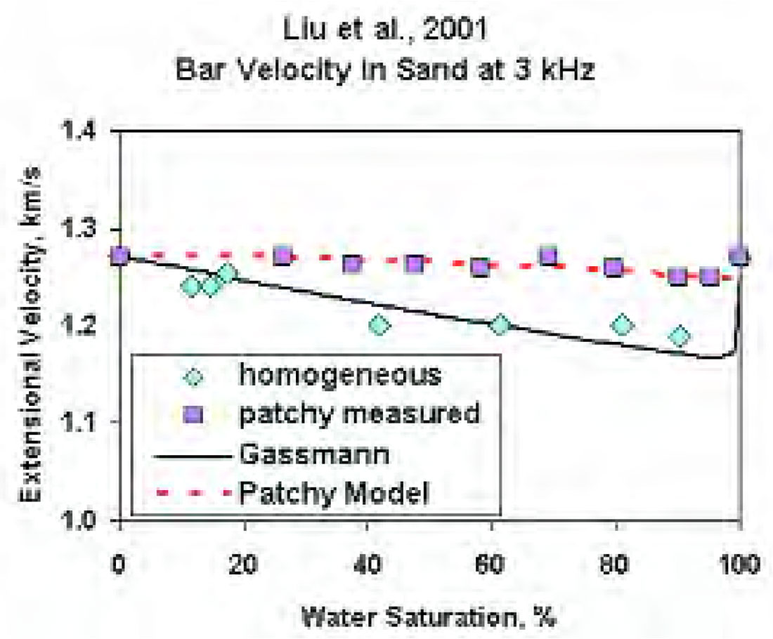
Gassmann theory assumes that all pore fluids are homogeneously distributed. For the special case where the reservoir fluids are not homogeneously distributed, pore pressures may not have time to equilibrate between adjacent fluid “patches” during a seismic or sonic event (that is, the pore fluids are not “relaxed”). This will cause the velocity to be higher than that predicted by Gassmann theory. Figure 1 shows an example of sonic-frequency measurements that agree well with Gassmann’s equation when saturations are homogeneous, and also agree with a patchy saturation model (see Mavko et al., 1998) when there are distinct wet and dry zones. Patchy saturation may arise during reservoir production or injection, or because of mud filtrate invasion while drilling.

A practical problem arises when fluid pressures are not equilibrated at sonic frequencies, but are equilibrated at seismic frequencies: how can wireline sonic data be used to predict seismic behavior? First the sonic data must be analyzed with a non-Gassmann theory, such as patchy saturation or the empirical model of Brie et al. (1995). Then Gassmann theory is used to estimate the saturated rock velocity at seismic frequencies. Some applications are described by Packwood and Mavko (1995) and Walls and Carr (2001).

Other Alternatives to Gassmann Theory.

Biot’s theory of poroelasticity (e.g., see Mavko et al., 1998) treats both high and low frequencies, and includes Gassmann theory as the low-frequency limit. Other theories exist which describe velocity behavior under special circumstances (e.g., “squirt flow” theory by Mavko and Jizba, 1991); most other theories are modifications of the more general Biot-Gassmann theory.

Ball et al. (2001), and Han and Batzle (2004) suggest a simple approximation to Gassmann’s equation in which the change in the bulk modulus of the rock is proportional to the change in the pore-fluid bulk modulus. The proportionality constant is basically a function of the porosity and the drained frame bulk modulus. This formulation makes computations a little easier and makes the physics a little more transparent.