The question for the ‘experts’ this month is on the determination of anisotropy parameters that may be subsequently used, during the processing of seismic data to include these effects. The experts answering the question are Ian Jones (GX Technology, UK), Rob Vestrum (Thrust Belt imaging, Calgary) and John Bancroft (University of Calgary). We thank them for sending in their responses.
The order of the responses is the order in which we received them.
Question
A common form of anisotropy observed in many geological settings is Transverse Isotropy (TI) where the reference axis or axis of symmetry is normal to the bedding surfaces. For simple layer-cake type models the symmetry axis is vertical and the anisotropy is known as Vertical Transverse Isotropy (VTI). Grain alignments in shales or repeated sequences of finely layered sediments (sand/shale alternation) are the primary causes for such anisotropy. Such anisotropy is usually quantified in terms of Thomsen’s parameters, ε and δ.
Many processing software algorithms are available today to handle such anisotropic effects. However, the difficulty in addressing anisotropy lies in the reliable estimation of parameters.
What are the different methods being used for the estimation of these parameters? You are requested to furnish at least one specific example to show the estimation of the parameters and how their use in processed output led to an improved result or calibration.
Answer 1
Although anisotropic data processing and migration have become more common over the past few years, the issue of anisotropic parameter estimation still remains contentious. In part, this problem stems from lack of sufficient data. To reliably obtain Thomsen’s delta parameter, we need well control, and to estimate the epsilon parameter, we usually require long offsets (offset ~ 2 depth). Occasionally, when we clearly see fault plane reflection energy intersecting sedimentary reflectors, we can also exploit these observations to help define the parameters.
Even when we have good data, correctly tying well markers to the correct seismic even can be ambiguous, and updating a velocity model based on higher-order moveout picks can be incorrect unless the geology is flat lying, or we have a good anisotropic tomographic inversion tool.
In the notes below, we’ll briefly consider four scenarios. Migrating with isotropic velocities; converting isotropic migration results to ‘true depth’, migrating with anisotropic velocities derived from isotropic migration velocities, and migrating with anisotropic velocities derived from scratch. It should be kept in mind that my own experience is primarily marine; dealing with the more complex foothills style of thrusted anisotropic units will bring its own challenges!
Isotropic Model Building
When we build a velocity-depth model for use with isotropic migration, we pick velocities which give rise to flat CRP gathers. In general, velocities from well logs cannot be used for migration, unless anisotropy is accounted for by the migration algorithm, and the degree (and type) of anisotropy known. The depth obtained in the conventional ‘isotropically derived’ velocity model will not generally tie well depths.
Well logs measure the vertical component of the velocity field, which tends to be lower than the horizontal component.
It is predominantly the horizontal component which is measured from surface seismic data. And it is this measurement which should be used to derive the migration velocity field, in order to collapse diffraction energy when we are running an isotropic migration. Occasionally, the well velocity can be higher than the seismically derived velocity (as in vertically fractured carbonates).
With a conventionally derived velocity-depth model, and isotropic migration code, if we want the resulting image to tie well-depths, we must perform an additional ‘depth conversion’ step. This conversion from ‘geophysical’ to ‘geological’ depth, usually involves converting the result of the isotropic depth migration back to time (using a smooth version of the isotropic model), scaling the interval velocities in the migration model to match the well velocities, then converting the ‘time’ data back to geological depth, with the well-calibrated velocities.
‘Depthing’ after Isotropic migration
The question does arise as to whether it is ’safer’ to migrate isotropically, and then convert to geological depth (calibrated to the wells) after the depth migration. In this case, we would have the trade-off between simplicity in the model building versus potential lateral positioning errors on steeply dipping events.
If the structure is not too complex, and the anisotropy not too pronounced, then ‘depthing’ after completion of isotropic preSDM may be acceptable (for laterally invariant elliptic anisotropy, epsilon = delta, depthing is an acceptable approximation). However, if the symmetry axis is tilted, this may not be acceptable.
Additionally, we may have a case where we have ambiguity in the parameter determination due to contributions from other factors which affect the depth and residual far-offset moveout but which may be erroneously interpreted as an anisotropic effect (e.g. vertical compaction gradients) Some of the travel time effects resulting from the gradient will be then be erroneously accounted for by incorrect determination of anisotropic parameters. For example, in an isotropic 1D medium in the presence of a strong vertical velocity gradient, preSTM using a straight-ray approximation will give rise to an apparent anisotropy with spurious eta values of about 20%. This is avoided for the most part by using a ray-traced (or curved-ray) preSTM algorithm.
Building an Anisotropic Model
(starting from isotropic velocities)
Sometimes we already have isotropic preSDM results, and want to perform anisotropic preSDM with the minimum of additional work. In this case, if the anisotropy is present primarily in one simple thick layer in the overburden, we can approximately adjust the isotropic depth model to be suitable for an anisotropic preSDM. We proceed as follows:
- Convert the isotropic depth model back to time via vertical stretch using smoothed isotropic velocities: this yields the isotropic ‘time’ model.
- Scale the interval velocity in the isotropic ‘time’ model, by dividing by (1+delta) (thus reducing the velocity for a positive delta)
- Convert the scaled time model back to depth. This will result in a model with shallower depth horizons and lower velocities (for a positive delta): in this new depth model, the depth horizons should (by construction) tie the well depths. This preserves the vertical travel time, but we commit an error by ignoring the lateral displacement associated with having (erroneously) determined the initial velocity field isotropically.
- Migrate anisotropically using the anisotropic velocity depth model from (3), and the associated delta values
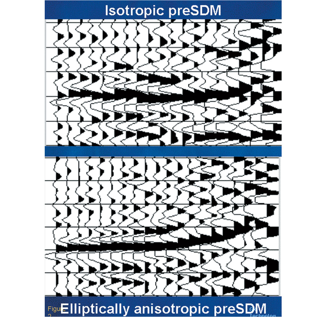
In figure 1, we see a CRP gather from the isotropic preSDM (top). In terms of conventional model building and CRP velocity analysis, we would be very happy with this result, as the gather is as ‘flat’ as it can be. However, after creating an anisotropic model by scaling the isotropic model (as described above) and running an anisotropic migration (using delta=10%, on the basis of well mis-ties), we get the picture at the bottom. Here we see that in addition to being ‘cleaner’, the CRP is also much flatter out to about half the offset range (full offset = 4200m), but then curls-up.
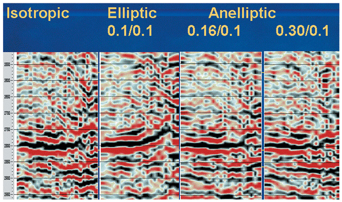
- We have now tied the well (for this horizon, the isotropic image was 178m too deep), but must estimate epsilon (for many shales, epsilon is typically about 2*delta). In this case, we ran a migration scan over possible epsilon values, some members of which are shown in figure 2.
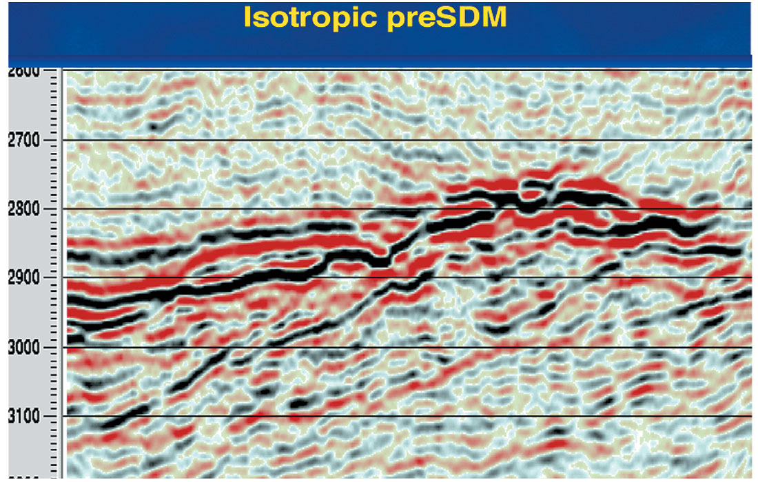
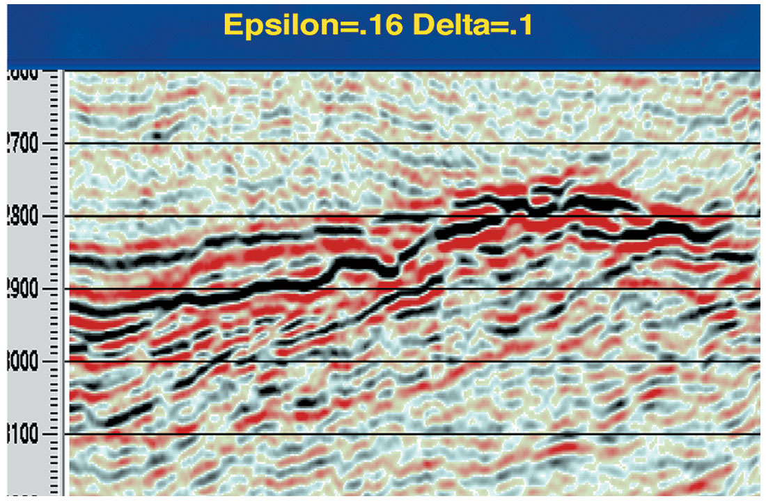
The images from the isotropic and anisotropic 3-D preSDMs are compared in figures 3 & 4 after conversion to time.
In this instance, a migration scanning technique was used to determine epsilon, after delta was measured from well mis-ties. However, if we observe consistent higher- order moveout effects on an horizon, after migrating anisotropically with delta (step 4 above) we can employ a continuous auto-tracker to pick higher order moveout (unfortunately, at high velocity contrast interfaces, we often get supercritical events which confuse the issue).
In the cases where we can employ an autopicker, we would:
- Convert the anisotropically migrated CRP gathers back to time, using the smoothed anisotropic model.
- Back-out the (second order) NMO using the associated RMS velocities if the initial migration used epsilon=0, OR back out higher order moveout with the given eta if a non-zero epsilon was used in the migration in step 4.
- Input these gathers to the continuous higher-order velocity analysis package, and analyse for higher-order moveout by measuring the eta parameter. Recall that it is Alkhalifah’s eta parameter that we measure from residual moveout in time gathers. Note that this is a cumulative eta value (also referred to as the ‘effective eta’). In order to obtain the interval values of eta, we must perform a Dix-style inversion first. To obtain epsilon for a depth migration, we then use the relationship η = (ε - δ)/(1+2*δ) to recover epsilon. It must also be noted that this inversion must account for the fact that the non-anisotropic elements of higher-order moveout have already been corrected (by ray-bending in the migration). In other words, we have solved for the geometric component of higher-order effects with the initial depth migration, and now want to resolve the anisotropic component.
Building an Anisotropic Model (starting from scratch)
In the case of a new project, especially in the presence of good well control, we can commence differently, performing a topdown anisotropic model build.
For very dense well control, we can:
- 1. Migrate data with the well-derived velocity field (in other words, we are already accounting for an initial estimate of delta).
- Scan for epsilon and delta values by applying residual moveout to gathers as a function of these two values. We will be correcting the implicit estimates of delta, and obtaining our first estimates of epsilon.
- Assign the values of epsilon and delta to the depth model
- Remigrate data and monitor both well-ties and flatness of gathers both laterally and horizontally.
Alternatively, we can run a dense autopicker to recover vertical compaction gradient information and then tomographically invert the picks to update the near offset component of the seismic velocity field. The ratio of the seismically derived velocities to the well-based velocities will be a first order estimate of the delta field (recall that Vnmo = Vvertical *(1+δ))
For relatively flat data, the delta parameter can be estimated from non-migrated data by employing depth conversion first on the basis of well velocities and then the seismic velocities (where the seismic velocities include vertical compaction gradients). The ratio of these estimates will yield an estimate of the delta field (as above).
There is also the issue of whether we permit lateral variation of the epsilon and delta parameters within a layer. More often than not, we lack the well control and long offset information to justify this, and to-date, we have hitherto used fixed epsilon & delta pairs for a given layer (this is not a limitation of software, but more of geophysical justification).
In addition, we have the issue of model representation: to implement anisotropic ray-tracing, we need to carry the dip vector for the surfaces bounding the anisotropic layer (for cases where the anisotropic tilt axis is normal to the layer). Thus for a gridded model, which at GXT we routinely use to carry the vertical velocity field, we need to also supply associated interpreted layers for the dip field. (In a gridded velocity model, the dip field is determined locally whenever a coherent velocity measurement is made, but this is less easy to use for the anisotropic parameterisation, hence layers are also employed.) For a purely layer-based model, this extra complication is not present. In cases where the anisotropic tilt axis is de-coupled from the seismic reflection interfaces (as it can be for some combinations of compaction and deposition), we still need separate ‘surfaces’ to carry the tilt axis information for a layered model.
Ian Jones
GX Technology, UK
Answer 2
Anisotropic parameter estimation for seismic data processing takes a variety of forms, depending on the geologic setting, type of seismic data, and the available model constraints. Inherent ambiguities in estimating anisotropic parameters from surface seismic data, as described in detail by Jones et al. (2003), require us to make some assumptions as to the geometry of the anisotropic strata and to utilize external constraints such as well depths. In this, my answer to Satinder’s question, I offer a cursory overview of recent work in estimating parameters for VTI anisotropic velocity models with a few of the key references to point the reader in a few directions for further study. In the light of the VTI overview, I address the problem of estimating anisotropy in a thrust-belt environment where the dipping anisotropic strata are modelled as TI media with a tilted axis of symmetry (TTI).
Parameter estimation for VTI moveout curves using higher-order moveout curves is well documented (e.g., Byun and Corrigan, 1990; Alkhalifah, 1997). Picking higher-order moveout terms will produce an improved seismic image and picking these higher-order moveout terms yield the moveout velocity and the anisotropic parameter η. What this process does not give us is the vertical velocity that we need for accurate depth conversion and we cannot separate out ε from δ, which are hidden in the η term for the VTI moveout equation.
Tsvankin and Thomsen (1995) demonstrate that, for P-P reflections in VTI media, there are a range of models with differing vertical velocities that each provide accurate traveltime curves. They successfully reduced the ambiguity of the anisotropic velocity model with a joint inversion of P-P and P-SV moveout curves.
Most of these methodologies and rules of thumb work well in the VTI case, where the anisotropic strata in the overburden has a horizontal orientation. However, the inherent traveltime and imaging assumptions break down and are invalid when applied to foothills seismic data, where the anisotropic overburden has arbitrary dip that ranges from 0° to 90°. When we have dipping beds, we assume that the primary axis of symmetry is tilted, and we then call the medium tilted transverse isotropy or TTI ( Vestrum et al., 1999).
In the TTI case, the additional complexity of varying dip of the overburden and varying reflector geometry makes it difficult, if not impossible, to derive analytical equations to predict traveltime curves that correct for anisotropic effects. Since the early days of my research into TTI imaging (Vestrum and Muenzer, 1997), I have taken the inverse-modelling approach to estimating the anisotropic velocity model.
Inverse modelling for TTI parameter estimation
We interpret an anisotropic velocity model from the prestack time migration and any other available geologic constraints, such as well logs, surface geology, and an understanding of the regional structural styles. The model is then used in anisotropic depth migration and the model is perturbed until we arrive at a model that yields an optimum seismic image with flat image gathers and a correlation to well depths.
The initial velocity model includes some non-zero values for the anisotropic parameters, ε and δ, because we don’t want to bias any velocity analysis with anisotropic parameters that are too low. If we perform seismic velocity analysis ignoring anisotropy, i.e., building a velocity model with ε = δ = 0, we will estimate velocities that are 8-10% higher than the true vertical velocity (Schultz, 1999) and therefore the depths to seismic reflectors will be greater than the depths to their correlated geologic horizons (Etris et al., 2001). I have found in practice over the last nine years of building anisotropic velocity models that ε = 0.12 and δ = 0.03 are reasonable initial values for imaging below interbedded sandstones and shales. By using moderate values such as these in the initial model, the velocity estimates from standard image-gather analysis will be much closer than the 8-10% velocity overestimate that we see when interpreting velocities while ignoring anisotropy.
The danger with the above paragraph is that some depthimaging practitioners have taken to using ε = 0.12 and δ = 0.03 as constant values for depth-migration velocity models in the Canadian foothills. I have had geophysicists ask me to justify my “claim” that all rocks in Canada have anisotropic parameters with these values. I have never made such a claim. I suggest these values as starting points because they will work better than the isotropic assumption, ε = δ = 0, and a depth imager will converge to an optimum velocity model with fewer model updates if he or she does not ignore anisotropy in the beginning of the model-building process. A process that produces the best seismic image and the most accurate well tie will include a reevaluation of the values of the modelled anisotropic parameters as the depth imager converges on an optimum velocity model.
Once we have an anisotropic depth migration from our initial velocity model, we are in the stage of the inverse-modelling process where we are continually re-interpreting our velocity model in hopes of improving the seismic image. We may then use standard image-gather analysis to see if our model velocities are too high or too low. In cases where image-gather analysis does not give us the full picture or where prestack signal-to-noise ratios are low, we perturb the model parameters, migrate, and compare final migrated sections looking for improvements in reflector continuity and amplitude.
Figure 1 shows the model-perturbation technique for values of ε and δ. The migrations with varying δ (Figures 1a, 1b, 1c) show some shift in the lateral position of the structures. Confidence in the value picked for δ translates into confidence in the lateral position of the target structure. Note here that the optimum image is not at δ =0.12 (Figure 1c), but it is at ε = 0.08 (Figure 1b). I have typically found that accurate correlation between well depth and seismic depth requires an increase in ε from the initialmodel value, but, in this case, a sandstone-dominated clastic overburden required a lower value of ε to yield an optimum image. Varying δ over the same interval (Figures 1d, 1e, 1f) shows a more subtle imaging change than we observed with varying δ. As with ε, an optimum value for δ is different from the initial-model value, only this time δ is larger than the initialmodel value; I chose δ = 0.08 (Figure 1e) as the optimum value.
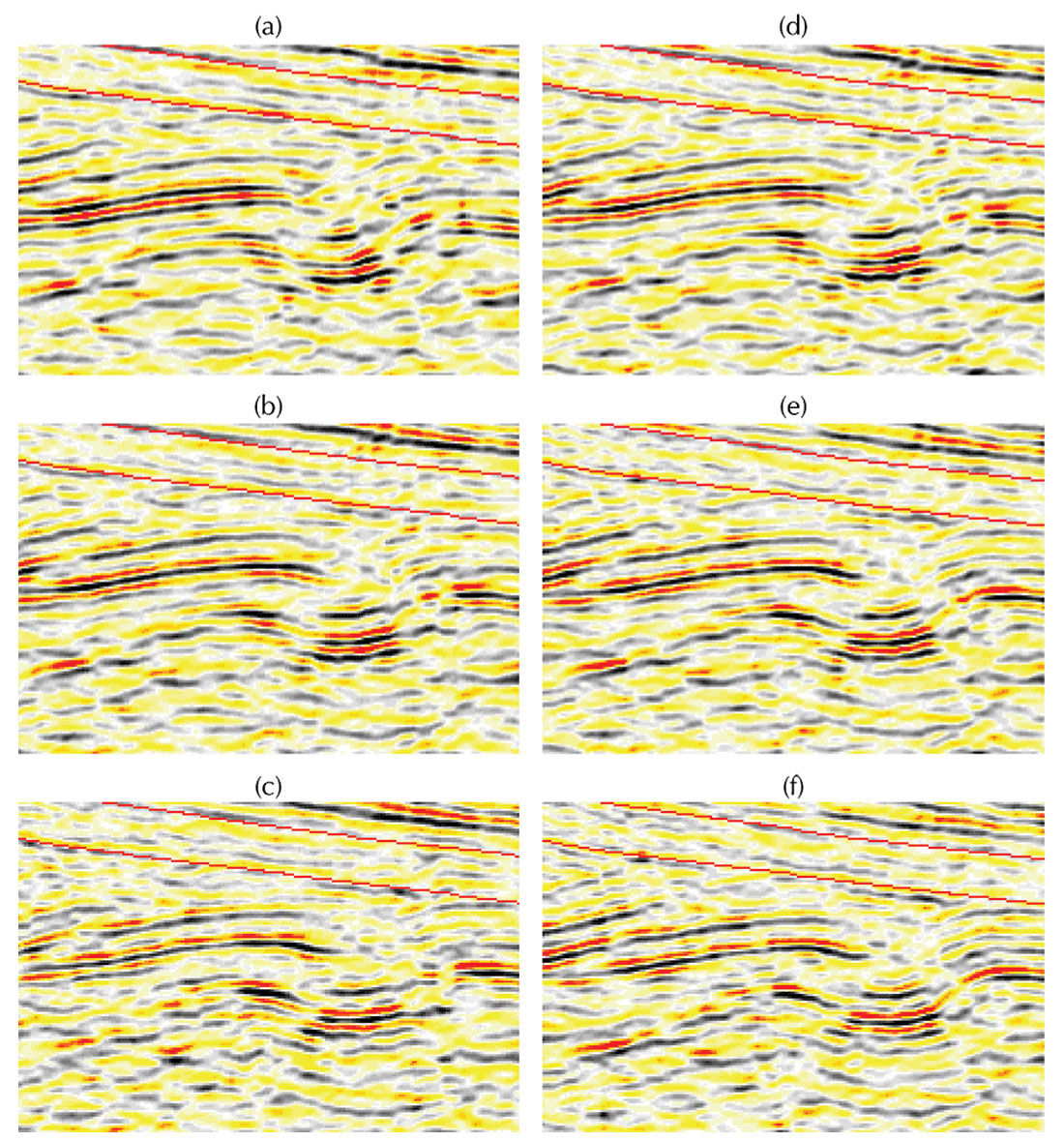
Figure 2 shows the well tie to the isotropic depth-migrated section (Figure 2a) and the anisotropic depth-migrated section (Figure 2b). I estimated the anisotropic parameters from using the method illustrated in Figure 1. Note that the isotropic depth migration has a reasonable image, but the seismic depth is deeper than the depth correlated from the well-log data, as predicted by Shultz (1999) and Etris et al. (2001). The anisotropic depth migration yielded depths on the seismic image within a half of a seismic wavelength.
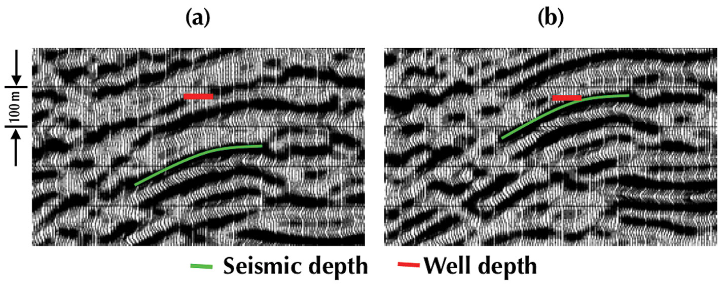
The example shown in Figures 1 and 2 is a rare example where we could estimate anisotropic imaging parameters with reasonable accuracy without additional model constraints. In most cases, accuracy of the model-building process does not satisfy the exploration objective and give enough confidence in the accuracy of the lateral position of the target image. Geologic depths from wells then provide an essential constraint on the anisotropic parameters of a velocity model. In the case from Figure 2, one might look at the well tie in Figure 2a and hypothesize that a lower velocity and a higher ε would raise the seismic reflector to a more accurate depth while preserving the quality of the seismic image. After a few parameter tests, one might then discover that the seismic image improves as the seismic reflector moves closer to the well depth (Figure 2b). With some additional effort, the seismic and well depths should match perfectly with an optimum seismic image. Once the depth imager meets these criteria, the seismic interpreter can then be confident in the depths of reflectors away from the well-calibration point and perhaps more importantly, confident in the lateral position of the target structures.
Future work
So far, most TTI model-building efforts have taken some form of inverse modelling similar to the method described above. Isaac and Lawton (2004) are looking at observable phenomena with lateral-position differences of target events on different offsets to ultimately invert for the anisotropic model in a TTI setting. Additional work here will include developing diagnostics based on these observations that may be used as constraints on the velocity-model interpretation.
An inverse modelling exercise is a great place to integrate multioffset VSP traveltimes as an additional constraint. Parameter inversion from VSP traveltime and joint migration of VSP and surface-seismic data has been done successfully by Grech et al. (2003). The next step here is to integrate forward modelling of VSP traveltimes into the depth-migration velocity-model interpretation.
Conclusions
Estimating anisotropic parameters from surface seismic data is inherently under constrained. Additional model constraints, such as shear-wave data, VSP traveltimes, surface geology, and reflector depths from well logs aid in the interpretation and/or inversion of an anisotropic velocity model. As we understand various anisotropic phenomena that we can observe on our seismic data, we will continually improve our estimates of anisotropic parameters used in seismic data processing.
Rob Vestrum
Thrust Belt Imaging, Calgary
Answer 3
Use of Thomsen’s parameters, ε and δ.
The first part of this question mentions some of the primary causes of anisotropy. I would like to add to these assumptions as they have different impacts on seismic processing algorithms. We will then mention a few measurement techniques, and refer to papers that have included anisotropy in prestack migrations.
Moveout (MO) correction is applied to offset data to align or flatten reflection energy with that recorded with zero offset, so that it can be stacked. In areas with horizontal stratigraphy, it is referred to as normal moveout (NMO), and in areas with structured or dipping stratigraphy it may be referred to as dip-dependent moveout (DD-MO) (historically referred to as dip moveout). Even in a constant velocity medium, DD-MO requires a higher stacking velocity than the velocity of the medium.
It is typically assumed that the shape of moveout energy in a common midpoint gather (CMP) is hyperbolic. MO correction equations with orders higher than a hyperbolic equation may be used to extend the offset range that can be flattened, and we may attribute this non-hyperbolic effect to anisotropy.
We have been able to ignore anisotropy for many years because compensating for its effect has been built into the stacking velocities Vstk. For example, if the anisotropic velocities are elliptical, then the moveout will be exactly hyperbolic and a processor will choose a velocity Vstk that will “flatten” the MO. Even when the anisotropy parameters are not elliptical, the shorter offset traces still exhibit a reasonable hyperbolic shape and can be successfully moveout corrected and stacked. A processor will not know that the anisotropy effects are included in the velocity analysis and may not be aware that the structure is dipping. Consequently, when processing azimuthally oriented velocities for 3-D seismic projects, a slight change in the dip will produce a change in velocity that may also be attributed to anisotropy, (Ye Zheng 2005).
Attributing all non-hyperbolic moveout to be caused by anisotropy may be permissable for stacking, post-stack time migration and even prestack time migration, but can cause severe problems with depth migration.
Consider the effect of non-hyperbolic moveout that is caused by a low- frequency trend of the velocity. In a medium where the velocity varies linearly with depth, V(z) = V0 + kz, all wavefronts and raypaths are circular. However the moveout shape from a discontinuity (say a change in density) will produce non-hyperbolic moveout that has a distinctive bell shape. At long offsets, this isotropic medium will appear anisotropic. Any isotropic depth migration would correctly honour the raypaths due to the velocity change. However, an anisotropic depth migration that incorporates the estimated “anisotropy parameters” will distort the raypaths, and in effect, apply the “anisotropic” effect twice. Therefore, care must be taken with anisotropic depth migrations to ensure that the moveout distortion caused by the low frequency velocity trend is not included when estimating the anisotropy parameters.
In a horizontally layered medium, we use the vertical interval velocities estimated from well logs, VSPs, check shots, or depth measurements, to compute the theoretically correct root mean square (RMS) velocities Vrms-1. These velocities define the curvature at the apex of the moveout curve, and thus they define the hyperbolic shape of the moveout for short offsets. In the absence of anisotropy and dipping reflectors, this RMS velocity should equal the stacking velocity Vstk , i.e., Vstk = Vrms-1. In the presence of dip (but not anisotropy), the stacking velocity for DD-MO is increased by the well known formulae

Unfortunately it has become common practice to use the RMS velocity term to represent the stacking velocity for horizontal layers, which I now defined as Vrms-2, and reserve the term stacking velocities for dipping structures. However, in the presence of anisotropic horizontal layering the stacking velocity is different from the computed RMS velocity Vrms-1, i.e.,

It is this difference between Vstk and Vrms-1 that is used to compute the anisotropy parameters.
The moveout velocity, when measured on CMP gathers is subject to the dip of the reflector (DD-MO) and produces corresponding errors in the anisotropy estimates. The equivalent offset method (EOM) of processing produces prestack migration gathers that are independent of the dip, contain a superior signal to noise ratio, and are located at the reflector. They are formed with minimal velocity information, but provide accurate velocities after they are formed. If anisotropic estimates are included when forming the gathers, the moveout in an EO gather will be hyperbolic for a simpler velocity analysis. For prestack time-migration processing, we can use the non-hyperbolic moveout estimates to either stack the data directly (without the need to know the anisotropy parameters), or estimate the parameters. For prestack depth migrations, the location of energy at the equivalent offset in the common reflection point gather aids in building an anisotropic velocity model that is structurally viable (Bancroft and Vestrum, 1999).
On the use of Thomsen’s parameters, ε and δ.
It is reasonable to assume the anisotropy is weak and that Thomsen’s (1986) parameters provide an adequate representation. However, there may be more convenient forms of these parameters such as (ε - δ) that have more practical meaning, as discussed by Daley (2002).
It is not until we compare the NMO stacking velocities Vstk, with the structure and with RMS velocities Vrms-1, (derived from well logs, check shots, VSPs, or depth conversions), that we become aware of the discrepancy, and may have attributed it to some “other” effect. It is this difference that now provides the basic estimate of P-wave anisotropy, specifically the parameter δ that was so well “hidden” in the stacking velocities, i.e.,

Estimation of the Thomsen parameters
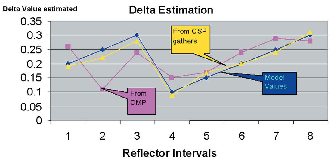
Higher order and shifted hyperbola equations are also used along with mode converted recording to estimate the other Thomsen’s parameters (Tsvankin and Thomsen 1994, Thomsen 1999, and Elapavuluri and Bancroft 2003). An example in Figure 1, from Elapavuluri and Bancroft (2003), compares numerical model values of δ with estimates using CMP and common scatterpoint (CSP) gathers. Table 1 then provides estimates of ε and δ for five horizons from real data collected at Blackfoot, Alberta, Canada.
| Formation | δ (estimated) |
ε (estimated) |
|---|---|---|
| Table 1. Estimates of ε and δ using EO gathers. (Elapavuluri and Bancroft 2003) |
||
| BFS | 0.23 | 0.06 |
| MANN | 0.04 | 0.008 |
| COAL | 0.24 | 0.12 |
| GLCTOP | 0.06 | 0.006 |
| MISS | 0.00 | 0.001 |
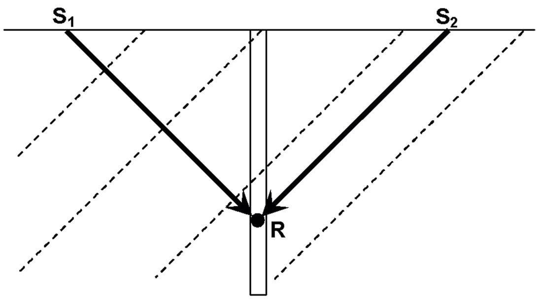
A considerable wealth of papers on estimating anisotropy parameters is contained in the archives of the F-FRP consortium at the University of Calgary. Some topics include the use of refraction and vertical seismic profiles (VSP) (Newrick and Lawton 2002), VSP’s in tilted transverse isotropic (TTI) media (Newrick et al 2002), or directly from seismic data (Isaac and Lawton 2004). Some of this work is based on a concept that is illustrated in Figure 2, which contains a borehole in tilted transverse isotropic media. The source S1 has a raypath to receiver R normal to the bedding while S2 has a raypath parallel to the bedding. Anisotropy measurements are obtained by comparing the traveltimes from S1 to R with the traveltimes from S2 to R.
The estimates of these anisotropy parameters are defined at specific location, but may be used (to first order approximations), to represent the parameters for the entire bed as it extends across the project. However, just as the interval velocity of a layer may vary with depth and dip, we can expect the anisotropy parameters to also vary with depth and dip. Consequently, anisotropy parameters measured from reflection seismic may have additional benefits, providing there is reasonable well control.
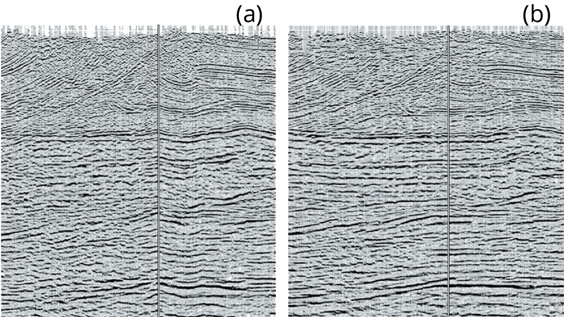
Comparison of isotropic and anisotropic depth migration
A comparison of an isotropic and anisotropic depth migration is displayed in Figure 3. The velocity model used for the anisotropic migration (b) was simpler to evaluate and more geologically reasonable than those used in the formation of (a) (Bancroft and Vestrum 1999).
Summary
- It is OK to use anisotropy estimates to compensate for non-hyperbolic moveout for stacking, and time migrations.
- Caution must be taken when using an anisotropic depth migration where the low frequency velocity trends may be included in an estimate of the anisotropy parameters
- Most estimates of the anisotropy parameters require borehole measurements.
- The inclusion of anisotropy effects improves the imaging and produces a velocity models that conforms to geological principles.
- Cautionary note:
Using longer offsets will improve the SNR of a stacked section, but the increased NMO stretch with the longer offset may reduce the resolution.
John Bancroft
University of Calgary, Calgary
Acknowledgements
I wish to thank the members of the CREWES and F-FRP consortiums for their generous help in the preparation of this material. We welcome your visit a www.crewes.org and www.geo.ucalgary. ca/frp/.


Share This Column