This issue of the RECORDER features a question that looks for answers for distinguishing ‘fizz water’ and ‘ commercial gas’ saturations and locating ‘heavy oil sand units’ with surface seismic and borehole data and the trends in this field.
The ‘Experts’ answering these questions are Zhijing Wang (ChevronTexaco), Michael Batzle (Colorado School of Mines) and De-Hua Han (University of Houston), and Tapan Mukerji (Stanford Rock Physics Project). We thank them for sending in their responses to our questions. The order of the responses given below is the order in which they were received.
Question
Distinguishing “fizz water” and “commercial gas” saturations and locating “heavy oil sand units” with surface seismic and borehole data are two challenging problems for us today. How are we meeting these challenges?
Answer 1
Theoretically, it’s nearly impossible to distinguish “fizz water sand units” from “commercial gas sand units”, or “heavy oil sand units” from “water sand units”, just using P-wave impedance or P-P reflectivity data. This is of course because “fizz water sand units” and “commercial gas sand units”, or “heavy oil sand units” and “water sand units”, have similar P-wave impedances (or the difference is so small that it is unresolvable seismically).
This is a tough problem as the exploration geophysics industry relies heavily on P-P reflectivity data and P-wave impedances and contracts to identify structures, stratigraphy, and potential fluids. As such, this problem is currently unsolved.
But how are we meeting these challenges? Potential research topics are
- Using very far (beyond 30°) offset data or elastic impedance: At far offset, seismic reflections are heavily influenced by not only the P-wave impedances, but also the S-wave impedances, the P-S impedance ratio, and density contrasts. As a result, very far offset seismic data could contain information on the amount of gas saturation, giving potential to distinguish “fizz water sand units” from “commercial gas sand units”. This of course depends on the quality of very far offset data and many other challenging factors. This is still a research/testing topic which I have not seen many success stories.
Very far offset data could also be used to distinguish “heavy oil sand units” from “water sand units” because heavy oil sands usually have higher S-wave velocities but lower bulk densities than water sands (unless reservoir temperature is below 17°C and the API gravity of the oil is less than 10). Because heavy oil sand units tend be shallow, far offset data can be easily collected. It would be much easier to distinguish “heavy oil sand units” from “water sand units” if reservoir temperature is raised. P-wave velocity increases in water (to 73° C) but decreases in oils as temperature increases, creating impedance contrasts not existing at low temperatures. - Using converted wave data: Besides far offset P-P reflectivity, P-S converted waves offer another source of information (or constraint). The theoretical concept is similar to using very far offset data: utilizing the S-wave impedance, the P-S impedance ratio, and density contrasts to distinguish “fizz water sand units” from “commercial gas sand units”, or “heavy oil sand units” from “water sand units”.
- Using scaling effect and attenuation: Most fluid substitution calculations are based on the Gassmann equation which assumes uniform gas saturation and “zero” frequency. In reality, gas in “fizz water” or “commercial gas reservoir” may be in “patches”. If the “patch” sizes are bigger than 1/10 to 1/5 of the seismic wavelength, gas saturation should then not be viewed as “uniform”. In this case, the “patchy saturation” formulation can be used to calculate gas-saturation effect on acoustic and elastic impedances. The “patchy saturation” scheme is simply an averaging or scaling method to accommodate the effect of heterogeneity on seismic wave propagation (heterogeneity is a relative term to seismic wavelength). When gas saturation is in patches, seismic impedances decrease systematically with increasing gas saturation. Depending on other factors like seismic resolution and offset, gas saturation could be quantified using seismic data, although much research is needed before successfully applying the patchy saturation scheme in the field to quantify gas saturation.
Literature data have shown that attenuation reaches a peak at 10-15% gas saturation in water-gas saturated sandstones. If “fizz water” saturation is in this range, it might be possible to use seismic wave attenuation as a tool to distinguish “fizz water sand units” from “commercial gas sand units”. However, if “fizz water” saturation is <10%, attenuation would not be able to distinguish “fizz water sand units” from “commercial gas sand units” (same attenuation on both sides of the peak). The biggest problem in attenuation measurement is accuracy – it is extremely difficult to get accurate attenuation measurements in both fields and labs. Again, much research is needed to understand the effect of gas saturation on seismic attenuation. - Using other seismic attributes: it could be possible to study other seismic attributes (e.g., spatial correlation, dispersion, wave-train geometry, etc.) to distinguish “fizz water sand units” from “commercial gas sand units”, or “heavy oil sand units” from “water sand units”. However, we need to understand the physical meaning of such attributes before coming up with concrete recommendations.
There must be more research efforts going on than what I am aware of. But in terms of rock and fluid physics, distinguishing “fizz water” from “commercial gas” saturations and locating “heavy oil sand units” with surface seismic and borehole data remain as two challenging problems for us today and tomorrow. Hopes lie on obtaining and using quality S-wave data, scaling and attenuation, and other seismic attributes. I do not see, however, any “silver bullets” in solving these two tough problems any time soon.
(I would like to thank Gopa De, Joe Stefani, and Bob Laing of ChevronTexaco for their review and input to this write-up).
Zhijing (Zee) Wang
ChevronTexaco Energy Technology Co.
Answer 2
Differentiating “fizz-gas” from commercial gas reservoirs
“Fizz-water” or “Fizz-gas” is a rather ill-defined and misused concept. Ask five people what fizz-gas means, and you will usually get ten different answers. For some, it refers to gas in solution of brine; for others, it is defined as small amounts of free gas phase. This small, uneconomic gas content then gives rise to seismic bright-spots or other Direct Hydrocarbon Indicators (DHIs). Unfortunately, it is often the culprit of choice when no other reason can be found for the false DHI which has been drilled. However, progress has been made in assessing the problem pre-drill, and several promising techniques, such as extended AVO and 1/Q analysis are being developed.
First, by examining the physics of the rocks and fluids, we can tell you what fizz-gas is not. Measured data show that dissolved gas has negligible effect on water velocity, modulus, or density. A free gas phase is required. In addition, gas bubbles exsolving from either water or oil have only a small effect on bulk fluid properties at pressures higher than about 20 MPa (about 3000 psi). Gas under the typical high pressures and temperatures of deep targets has properties similar to light oil. This requires a much larger gas content (in some cases, more than 40%) to cause the same effect as a few percent gas under very shallow conditions. Part of the problem here may be the influence of invaded mud filtrate, which would result in lower apparent gas contents.
Other indicators are now being developed to address fizz-gas discrimination. Russell et al. (2003) summarized the DHI techniques associated with AVO. The indicators can usually be reduced to a form dependent on the difference between the compressional and shear impedances: Z2p-CZ2s, where C is a calibration constant. Dillon et al. (2003) pointed out that the value of this constant C is important in maximizing the hydrocarbon discrimination (and is often larger than the values suggested by us rock geeks). For deep-water unconsolidated sand reservoirs, a high-pressure gas is similar to light oil. At deep-water conditions, modulus and density of gas tend to be high, but can vary over a wide range. We actually have a chance to differentiate a gas reservoir from a fizz gas zone, if we can carefully calibrate the seismic parameters as shown in Figure 1.
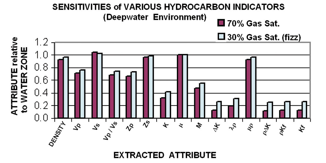
Attributes such as modulus K, fluid factor ΔΚ, λρ, ρ*ΔΚ, ρ*Κf, and Κf, illustrate significant differences between fizz and gas reservoirs. A fizz-gas zone has significantly different values of these attributes than those of a gas reservoir. All these attributes are mainly controlled by fluid modulus Kf. We need better methods to calibrate seismic attributes not only on gas zones, but more importantly in brine zones to give us background calibration. Forward modeling, with accurate rock and fluid properties, and reservoir structure (include fluid distribution), is also a powerful tool to quantify hydrocarbon indicators.
With different reservoir environments, identifying gas reservoirs may be more difficult and will require accurate local calibration (& forward modeling) to identify the best hydrocarbon indicators. At issue is how sensitive seismic waves are to variation of gas saturation for the target reservoir. Here we summarize some cases in Table 1:
| Lithology | Risk factors | Influencing factors | Gas indicators |
|---|---|---|---|
| Table 1. Different cases of gas reservoirs with different gas indicators. | |||
| Shallow- loose | Seal, thin layers | Trap, seal, thick sand | ρ, μρ |
| Deep-loose sands | Thin layers | Over pressure | Κf, ΔΚ, Κ, λρ, ρΔΚ |
| Consolidated sands | Low f | Less cement, more cracks | Κf, ΔΚ, Κ, λρ, ρΔΚ |
| Carbonate | Low ϕ & permeability | Porosity, fractures | Low Vp,… |
| Shale, chert… | Low ϕ & permeability | Porosity, Permeability | Low Vp,… |
In the future, attenuation (1/Q), or frequency content, might prove a helpful attribute. Less is understood of 1/Q, but several researchers recently have reported success in using frequency content as a discriminator of hydrocarbons. In this case, fluid properties, distributions, and mobilities all contribute. However, the in situ fluid distributions and mobilities are often unknown. In addition, even the controlling mechanisms of attenuation are not well understood.
To locate heavy oil sands with surface seismic data seems not a problem because most heavy oil reserves have been found a long time ago. However, how to produce heavy oil economically and efficiently remains a real challenge. From a production point of view, to “locate a sand zone” means differentiating a production zone from shale and other flow barriers. However, heavy oil production is more complicated than lithology characterization. We would to address the different aspects of the problem from this production point of view.
Challenges to managing heavy oil production
Heavy oils are an enormous resource, and the difficulty in producing them efficiently suggests that geophysical monitoring could make an enormous difference. Continuous seismic monitoring may be the only way to help understand how to produce heavy oil efficiently. Most targets are shallow, so seismic data could be high frequency and high resolution, with dense coverage and large offset angles. Numerous wells may be available for calibration. However, several basic problems confront our application. These include poor characterization of the reservoir, changing rock characteristics, and fluids that are difficult to distinguish from solids.
In most seismic interpretation, the rock matrix is assumed to be about constant, with only small changes associated with changing pressures and fluid types. However, heavy oil deposits are often very friable sands, basically floating in the tar (the material is difficult to retrieve and test). After a process such as steam flooding, the matrix alteration could be the largest contributor to any observed time-lapse signature. Permeability of heavy oil sand also needs to be examined. However, the viscosity of heavy oil is so high, that intrinsic permeability may not be directly relevant to oil flow. How the steam invades, tension fractures caused by pore pressure increases, development of ‘worm’ holes, and pattern of heat transmission is probably more relevant. At this point, we often lack a basic understanding of these physical processes.
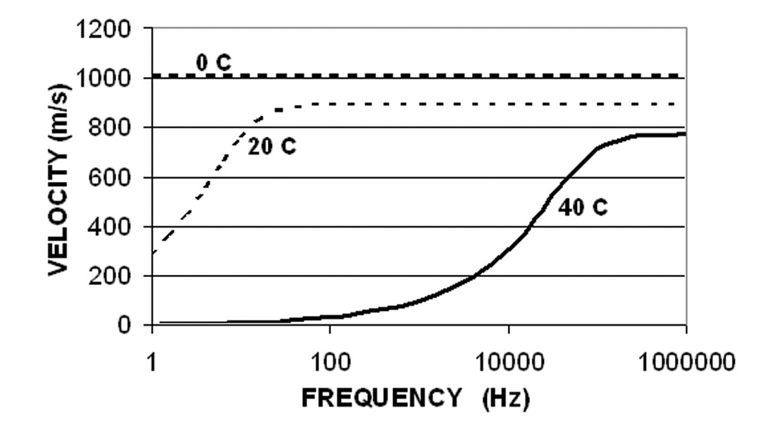
The heavy oils themselves are also different from most hydrocarbons. The dense oils are mixtures of complex compounds resulting from biodegradation. The extremely high viscosity and semi-solid nature adds a strong viscoelastic component to the seismic properties. Ultrasonic laboratory measurements will give higher velocities than sonic logs, which in turn will yield higher velocities than seismic data. Calculated values for shear velocity are shown in Figure 2. Heavy oils can have a substantial shear velocity, but this velocity is strongly frequency and temperature dependent. Highly dispersive velocities also mean high viscous losses in our seismic waves. These factors have not been fully investigated. They could be significant barriers to imaging heavy oil reservoirs efficiently.
Although the gas content of most heavy oils is low, small amounts of gas coming out of solution can have a major impact on the seismic and flow properties (we are back to fizz-gas!). Either pressure or temperature changes can force the oil across the bubble point. The influence of gas under such shallow conditions can be so strong that time-lapse monitoring may be monitoring only the bubble point moving through the reservoir, rather than, say, a thermal front. In addition, due to low gas pressure and relatively high viscosity, these bubbles of gas tend to stay mixed with the oil to form ‘foamy’ oil. Engineers have considerable information on the viscosity, compressibility, and gas-oil ratios of heavy oils. We must now translate and incorporate this information into our geophysical interpretations.
We also need to understand the nature of heavy oil production. Even good reservoir characterization is not enough to predict how the reservoir performs, especially as steam at high pressures and temperatures invades from the well. As we have seen, heavy oil at low temperatures (most cases in Canada) is in a solid or semi-solid state. Differential pore pressure is no longer as dominating a driving force with ‘solid’ oil flow. Therefore, basic flow patterns of heavy oil depend strongly on the specific design to heat the reservoir. However, local inhomogeneities such as shale breaks and flow barriers can also affect how the steam (heating agent) and heavy oil flow, and can be disruptive to well placement and design of surface facilities. We need better reservoir characterization on a local level. However, resolution of seismic data is often reduced due to near surface conditions. High-resolution lithologic identification is also needed. This identification may be helped by the longer offset angles possible with these targets.
The good news is that with proper characterization of reservoirs, lithologies, and fluids, and with a thorough understanding of the production process (using numerous monitor wells), we may grasp what is going on in these reservoirs and improve the efficiency of heavy oil production.
Mike Batzle,
Colorado School of Mines
De-Hua Han,
University of Houston
Answer 3
Distinguishing low gas saturations from commercial gas saturations
Attempting to seismically differentiate homogeneously mixed fizz water with low gas saturation from higher gas saturations is difficult. One of the most notorious pitfalls of AVO analysis is related to residual gas saturation due to leakage of a reservoir unit previously characterized by high gas saturation or low gas saturation due to gas coming out of solution from water or oil, caused by pore pressure drop (i.e., fizzy gas). The problem in AVO analysis is that residual gas saturations will yield similar seismic properties as commercial gas saturations. It should be noted that according to Han and Batzle (2002) fizz-water is an ill-defined and mis-applied concept. They found that dissolved gas or gas coming out of solution from water or oil at pressures higher than 20 MPa has little effect on effective fluid properties. This conclusion was based on experiments showing that dissolved gas coming out of solution at high pressures (>20MPa) has a negligible effect on total gas-water mixture compressibility because the exsolved gas has very small volume and high density at those high pressures. Hence, low gas saturation should have large effects on seismic properties only in shallow formations with low pore pressures. It is important, however, to bear in mind that significant residual gas may occur at pore pressures greater than 20MPa. If for example, a gas reservoir formerly filled with high gas saturation has leaked, leaving only a few percent of gas, we could still observe a significant drop in P-wave velocity, even at pore pressures greater than 20MPa.
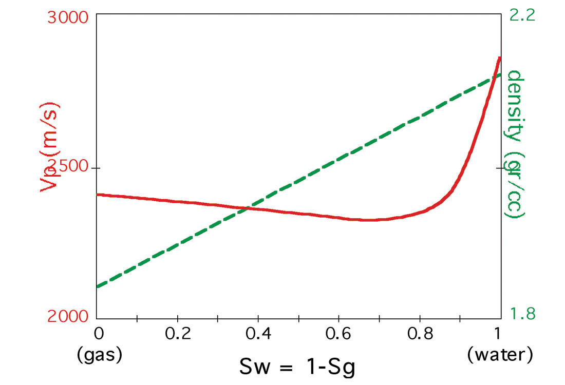
The abrupt reduction in VP with the first few percent of gas controls the P-wave seismic response (Figure 1). This effect is described by the Gassmann theory, assuming a uniform or homogeneous saturation distribution. Just a few percent gas will cause a significant drop in the effective fluid modulus, and consequently a significant drop in the saturated bulk modulus of the rock. Therefore, usually only the presence of gas but not the saturation can be detected with P-wave seismic. Notice in Figure 1 the abrupt jump in VP with the initial presence of a small amount of gas. In contrast the density varies more gradually and linearly with gas saturation. At low frequencies (surface seismic) the shear modulus does not vary much with gas saturation. As noted by Berryman et al. (2002) the linear behavior of density with saturation makes attributes that are closely related to density useful proxies for estimating gas saturation.
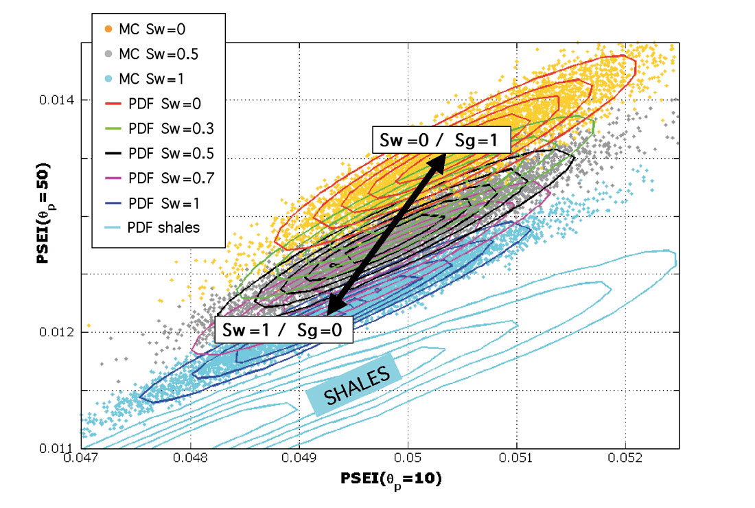
One approach (discussed shortly) is to use three-term, far-offset AVO to estimate density. Another promising approach (Gonzalez et al., 2003) is to use a converted-wave elastic impedance attribute (PSEI) that is closely related to density, and hence can be a good proxy for estimating saturation. Gonzalez et al show that at near offsets (small angles) VS and density terms contribute equally to PSEI. On the other hand, for mid-to-large offsets the density term dominates PSEI behavior. The asymmetric contribution or “decoupling” between the roles of Vs and density in PSEI can be exploited in discriminating different saturations. Figure 2 (from Gonzalez et al.) shows computations of PSEI at two different angles (or offsets). Values of PSEI monotonically decrease with reduction of gas concentration. Hence there is a real possibility of discriminating between different homogeneous gas saturations. An advantage of using two PSEI attributes, instead of a combination of PP-PSEI is that the PP and PS data time matching is avoided. The formulation of Gonzalez et al. uses PSEI in conjunction with statistical rock physics techniques to show the possibility of discriminating fizz water from commercial gas. Use of P-to-S converted waves (PS) has also been suggested as a source of additional information by Wu (2000), and Zhu et al (2000) for distinguishing high vs. low gas saturation.
Generally, 2-term AVO will not be able to discriminate a seismic anomaly caused by a few percent gas and an anomaly caused by commercial amounts of oil. This is found to be a universal problem, and many wells have been drilled on AVO driven prospects that indicated hydrocarbons, but proved to be residual amounts of gas. These were scientifically correct but commercial failures.
Density is probably the only elastic seismic parameter that can discriminate residual gas saturation from commercial saturation, because low gas saturation should imply bulk densities similar to 100% brine saturation, whereas commercial gas saturation should result in a significant drop in bulk density. In principle, density can be derived seismically from three-term AVO. Examples of the use of three-term AVO to calculate density include the papers by Kabir et al. (2000), Roberts et al. (2002) and Buland and Omre (2003), among others. A complicating factor in using density to discriminate residual gas saturation is the porosity of the reservoir. A sandstone unit with relatively high porosity and residual gas saturation will have similar density as a sandstone unit with relatively low porosity and commercial amounts of gas. Statistical classification techniques may help to reduce this problem. Chen et al. (2001) pointed out, as demonstrated by Swan (1993), that the method of calculating density from three-term AVO is very difficult because of the poor signal to noise ratio of the third term coefficient, which they referred to as the curvature term. A complicating factor that adds uncertainty to this procedure is the effect of anisotropy, which starts to dominate the reflection coefficient at mid to far offset ranges. Cambois (2001) argued that if the effects of anisotropy are mild enough to be neglected, the aperture is sufficient, and the S/N ratio is exceptional, reliable estimates of density contrasts may be obtained from the three-term Shuey equation. However, there are additional sources of errors beyond anisotropy that can make density calculations unreliable, including acquisition (source directivity and array responses become more significant) and processing effects (the parabolic assumption for multiples is not valid) on wide-angle data. Studies indicate that AVO parameter estimation from long-offset AVO based on exact Zoeppritz equations is a very unreliable procedure. Hence, full elastic waveform inversion should be applied to invert ultra-far seismic amplitudes for elastic properties. However, such an inversion is highly non-unique, and very computer intensive, making the procedure not yet practical for full 3D inversions.
Alternatively, another intriguing possibility is the use of attenuation to discriminate residual gas saturation. It is known from both experimental and theoretical rock physics that partial gas saturation will give larger attenuation than both commercial gas saturation and no gas saturation. Figure 3 from the pioneering experimental laboratory work of Murphy (1982) at Stanford University shows a peak in attenuation (inverse Q) at Sw of about 80%. Dvorkin et al. (2003a, b) have used modified versions of the patchy-saturation models of White (1975) and Dutta and Ode (1979) to theoretically quantify attenuation in partially saturated rocks. However, the technology of reliably estimating attenuation from seismic data is still immature, and few examples have been published in the literature showing successful applications of attenuation attributes for quantitatively estimating gas saturation. Challenges include separating scattering attenuation from intrinsic attenuation and relating the intrinsic attenuation to gas saturation.

Heavy Oil: Heavy oils represent a substantial resource. However we understand very little about the seismic properties and rock physics of sediments with heavy oils. The usual rock physics models of porous saturated media probably cannot be directly applied. Viscosities are very high, strongly temperature dependent, and below a certain transition temperature (around 40°C) heavy oils behave almost like a solid, supporting shear wave propagation (Batzle et al., 2004). This phase transition has obvious implications for the standard Gassmann fluid substitution recipe. At low temperatures (below 40°C) traditional Gassmann fluid substitution for heavy oils is certainly not valid any more. But is it valid at high temperatures when the heavy oil is more like a fluid with negligible shear modulus? Perhaps for low wave frequencies (such as surface seismic) it might still be OK to use Gassmann’s equations, provided the temperature is high enough (~above 80°C). There is also the important issue of the basic properties (compressibility and density) of the heavy oils. The popular and widely-used Batzle-Wang relations for hydrocarbon properties are based on empirical data and results that do not include heavy oils. Strictly speaking the published Batzle-Wang relations cannot be extrapolated to heavy oils, though preliminary computations show that the extrapolations may not be too bad for moderately heavy oil. It is believed that relations similar to the Batzle-Wang relations do exist for heavy oils, but these results have not yet been published in the open literature. How do we model sediments saturated with a highly viscous fluid? The heavy oil becomes almost a part of solid skeleton, acting like a cement between the grains. Leurer and Dvorkin (1998) have presented a theoretical model to estimate the effective elastic moduli and attenuation of granular material with a viscous cement.
Another very important and poorly understood aspect of heavy oils is “foamy oil” behavior. The release of dissolved gas, as pressure drops below the bubble point, is a key drive mechanism in the primary production from live heavy oil reservoirs. Unlike conventional oils, in the viscous heavy oil, the gas bubbles do not readily form a continuous phase, but remain trapped for a significant amount of time, forming a gas/oil dispersion or foam. The trapped bubbles help to increase flow and are critical for the recovery process. Foamy oil flow exhibit properties very important for the reservoir exploitation economics such as very high well productivity (in some case more than 10 times the predicted non-foamy flow rates); long duration (several years) of the foamy behavior in the reservoir; very high primary recovery factors (10-20 % instead 3-5 %); and a very good pressure maintenance (Maini, 1999, 2001).
As pressure gradually decreases below the bubble-point pressure, the reservoir reaches a maximum gas saturation when the average pressure of the reservoir has decreased down to the so-called “pseudo-bubble point” pressure. Below this average pressure the gas production becomes very high and the solution-gas drive looses its thrust. The gas bubbles coalesce and gas starts flowing as an independent phase, with typically high mobility. At this moment the reservoir engineer needs to select and to implement new reservoir production mechanisms such as steam or water injection.
Can this foamy oil behavior be monitored seismically? What are the seismic signatures of foamy oil flows? How does the dispersed gas, trapped by the heavy oil, change the elastic properties of the saturated rock? In an attempt to address some of these questions Maldonado and Mukerji (2002) made some simple (perhaps too simple?) calculations based on Gassmann’s fluid substitution recipe, with estimated gas saturations, as pressure drops from bubble-point to pseudo-bubble point. They estimated rock and fluid properties for a typical foamy oil reservoir from the Cerro Negro Block reservoir of the Orinoco Oil Belt in the Eastern Basin of Venezuela. The 8.5 API average crude is produced from unconsolidated Miocene sands with a reservoir temperature of 55-60°C. As discussed above, Gassmann’s relation may not be appropriate for heavy oils, specially at very low temperatures (below 40°C). However one might argue that for the Cerro Negro foamy oil Gassmann’s equation may not be too bad of an approximation because of two factors: a) the reservoir temperature is not too low, and b) perhaps the presence of dispersed gas bubbles makes the heavy oil behave more like a fluid with very low or zero shear modulus, at least at surface seismic frequencies. These are debatable points, but given the caveats, the calculations of Maldondo and Mukerji show that there can be up to a 28% change in P-wave velocity for unconsolidated sand reservoirs with foamy oil, as pressure drops from bubble-point to pseudo-bubble point. Even if the 28% change is off by a factor of three, it seems that foamy oil behavior might be seismically monitored at least for very unconsolidated sands with strong fluid sensitivity. Seismic monitoring of foamy oil would provide a critical guide for reservoir engineers planning and optimizing production strategies in heavy-oil reservoirs.


Share This Column