For the ‘Expert Answers’ this month, we posed the following questions on seismic data acquisition to two geophysicists, well known for their expertise in this area. The first question is about the choice of an optimum field geometry for a given subsurface target. The second question has to do with wide-azimuth and wide-offset data acquisition. These two questions were answered by Gijs Vermeer from 3DSymSam – Geophysical Advice, Netherlands and Mike Galbraith from GEDCO/SIS Software, Calgary.
Questions
1. The bin size, fold coverage or offset distribution may not be sufficient to determine whether a given geometry for a 3D survey would produce an optimum image quality in terms of resolution, reduced noise levels and accuracy in amplitude levels. In your expert opinion, how do you recommend on deciding on the most optimum geometry for a given target (yet be economical)? You may choose specific examples to illustrate your point of view.
2.Wide-azimuth and wide-offset data acquisition is required for reliable fracture characterisation. Another desirable feature is a dense and uniform offset and azimuth sampling in 3 dimensions. Are such 3D geometries feasible today; are they being used; could you furnish an example (synthetic or real)?
Answers by Gijs J.O. Vermeer
Question 1 consists of three parts: the first sentence describes the objective of 3D survey design, the second sentence poses the actual question and the third sentence gives some encouragement to provide examples.
The first sentence suggests that the objective of 3D survey design is to achieve optimum image quality. The optimum image quality is expressed in sufficient resolution, reduced noise levels, and amplitude accuracy. Indeed, each of those three aspects of image quality plays an important role in survey design. The sentence also suggests that the attributes bin size, fold of coverage and offset distribution of a particular design are not sufficient to judge the quality of the end product. Agreed again. But what then? That’s what the second sentence asks: How do you decide on the optimum geometry? The short answer to this question is: that is the design process, step-by-step (hopefully logical) reasoning to arrive at the optimum geometry. In my case, that design process is based on symmetric sampling principles.
Based on this interpretation of the first question, this Expert Answer should describe the design process. But how long should my contribution be? Apart fro m numerous papers written on survey design, even books have been filled on this subject (Stone, 1994; Liner, 1999; Cordsen et al., 2000; Vermeer, 2002). Obviously, it is quite impossible to cover all relevant considerations in just a few pages. Therefore, I must concentrate on some important aspects only and I will focus on the mechanics of the design process. Elsewhere, the philosophy of the symmetric sampling approach is highlighted (Vermeer, 2004).
My approach to survey design is first to choose the type of geometry, then to use a quick and simple technique to arrive at initial parameters of the geometry, and finally to fine-tune the quick solution in order to ensure “the optimum image quality”.
Geometry choice
I will assume that the survey will be a land survey. The most economical geometry for land is a crossed-array geometry (brick-wall, slanted, zigzag, or orthogonal), and the best of all crossed-array geometries, regardless the problem, is orthogonal geometry. So, we have to establish parameters for this geometry.
Outline of a simple approach to parameter choice
Geophysical information and geophysical requirements have to be translated into an optimal choice of parameters. On top of that, the parameter choice should also satisfy budget constraints. Therefore, choosing parameters for a 3D geometry can be considered an optimization process. In Vermeer (2003) I describe various geophysical requirements in more detail and I present modifications of the optimization methods proposed by Liner et al. (1999) and Morrice et al. (2002). In this part of my answer to question 1 I will outline a simple approach to survey design based on my 2003 paper with some extensions for points not entirely covered there.
Shot and receiver station intervals should be the same, as these have to satisfy exactly the same sampling requirements and (prestack) imaging would suffer from unequal sampling intervals (unequal sampling intervals are only acceptable in case of oversampling of one or both variables). The desired orthogonal geometry is defined by the station interval Δ and by the following four integers:
- nS, the number of shot positions between two receiver lines,
- nR, the number of receiver positions between two shot lines,
- Mi, inline multiplicity or fold,
- Mx, crossline multiplicity or fold.
These integers determine the shot line interval SLI = nR * Δ, the receiver line interval RLI = nS * Δ, maximum inline offset Xmax,i = Mi * SLI, and maximum crossline offset Xmax,x = Mx * RLI.
The geophysical input needed for a simple design consists of a representative velocity function, maximum NMO stretch factor, one to three target levels and for each level the required fold, required maximum frequency fmax (alternatively, required resolution), maximum dip angle θdip, and maximum angle used in migration θmig. The NMO stretch factor and the velocity function determine the mute function. The mute function in turn determines fold as a function of time or depth for levels where the full range of offsets is not reached due to muting. The velocity function is also used to establish the interval velocity Vint and the mute offset Xmute at the target levels.
To satisfy aliasing and imaging requirements at target level, the station interval Δk for target k should not be larger than

To satisfy aliasing and imaging requirements at all target levels, the station interval should be selected not larger than the smallest of all Δk ’s.
Feeding the required station interval, the mute offset for every target, and fold for every target into the optimization procedure described in Vermeer (2003) produces a value for each of the four integers nS, nR, Mi, and Mx.
Example
| Min.depth | Mid.depth | Max.depth | |
|---|---|---|---|
| TABLE 1 TARGETS AND THEIR MAIN PARAMETERS | |||
| Depth | 2000 | 2500 | 3000 |
| Required fold | 40 | 50 | 60 |
| Migration aperture (degrees) | 30 | 30 | 30 |
| Max. dip angle | 10 | 10 | 10 |
| Max. frequency | 70 | 70 | 70 |
| Max. station interval | 39.6 | 41.5 | 51.8 |
To illustrate the method of finding a quick solution, I will use the problem discussed at the 1999 EAGE Workshop, where a number of survey designers presented their solution to the same design problem (Hornman et al., 2000). Figure 1 shows the velocity function used for the design and Figure 2 the corresponding mute function for a maximum stretch factor of 1.15. These figures were made with the Acquisition Design Wizard, a simple interactive program that can be quite helpful in designing a 3D survey.
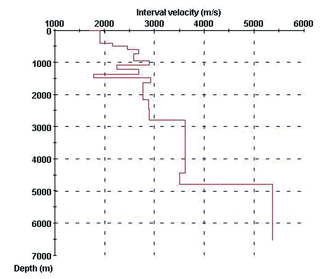
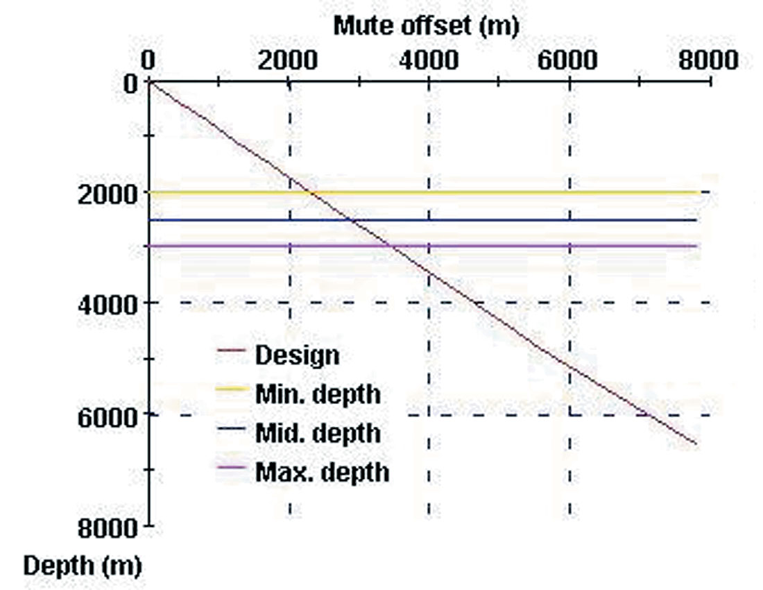
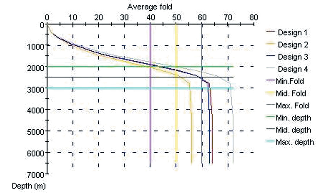
Table 1 shows parameters for the three target levels, including the desired fold at each level. The bottom row lists the maximum station intervals computed according to Equation (1). Given this information the Wizard proposed Design 1 shown in Table 2. It shows a fully symmetric design with folds at the target levels that exceed the required folds. The Wizard also provides Designs 2, 3 and 4 which are small permutations of the symmetric design. For instance Design 3 shows about the same fold as Design 1, but it achieves this with a larger shot line interval. Figure 3 shows a comparison of the fold as a function of depth for the four designs. The Wizard also provides parameters for AVO and for the fringe of the survey (not shown).
The mute offset for the three targets found in Figure 2 may also be used as input to one of the optimization procedures described in Vermeer (2003).
| Design 1 | Design 2 | Design 3 | Design 4 | |
|---|---|---|---|---|
| TABLE 2 PARAMETERS OF 4 DIFFERENT SOLUTIONS TO DESIGN PROBLEM | ||||
| nR | 8 | 9 | 9 | 8 |
| nS | 8 | 8 | 7 | 7 |
| Inline fold | 8 | 7 | 7 | 8 |
| Crossline fold | 8 | 8 | 9 | 9 |
| Station interval | 39 | 39 | 39 | 39 |
| Source line interval | 312 | 351 | 351 | 312 |
| Receiver line interval | 312 | 312 | 273 | 273 |
| Maximum inline offset | 2496 | 2457 | 2457 | 2496 |
| Maximum crossline offset | 2496 | 2496 | 2457 | 2457 |
| Fold | 64 | 56 | 63 | 72 |
| Largest minimum offset | 441.2 | 469.6 | 444.7 | 414.6 |
| Smallest maximum offset | 3088.6 | 3034.0 | 3034.0 | 3088.6 |
| Largest maximum offset | 3529.9 | 3502.4 | 3474.7 | 3502.4 |
| Fold at min depth | 42.8 | 38.0 | 43.5 | 48.9 |
| Fold at mid depth | 59.2 | 52.1 | 59.0 | 67.0 |
| Fold at max depth | 64.0 | 56.0 | 63.0 | 72.0 |
Discussion and fine-tuning
Choosing the parameters of orthogonal geometry using the simple procedure described above is adequate in many cases. Attribute analysis of midpoints is entirely superfluous, because one cannot do better than choosing a geometry that is square or nearly square. However, there are still some points needing further consideration.
Station interval. Especially the choice of station interval resulting from the simple approach needs to be checked carefully. The station interval obtained in this way is usually not small enough to guarantee alias-free sampling of the desired wavefield. It is likely, that interval velocity at shallower levels will be smaller needing smaller station intervals. Usually, this aliasing is taken for granted. However, if shallow levels generate many diffractions interfering with the target levels deeper down, it should be considered to use a smaller sampling interval for a sufficient cleanup of those target levels.
An entirely different approach to sampling is the single-sensor approach requiring much smaller sampling intervals because shot-generated noise is no longer suppressed by field arrays. In Vermeer (2001) I suggest that the move in land data acquisition to sampling intervals in the range of 5 to 8 m might skip a phase with 20 to 25 m shot and receiver station intervals with corresponding field arrays. This is still valid today with commonly used station intervals of 40, 50, or even 60 m (shot station intervals are often even larger). 20 or 25 m station intervals are in general not necessary for alias-free sampling of the desired wavefield (unless a very shallow target is illuminated with frequencies above 100 Hz). However, these station intervals may be selected to make noise removal much more successful than possible with larger station intervals and longer arrays.
Fold. Choosing what fold you need for the various target levels is still quite a subjective task. The choice has to be based on experience, knowledge of the area, what fold was needed for 2D lines in the area, etc. Moreover, required fold depends on the choice of station interval. Usually, the smaller the station interval, the lower the fold can be, because more noise can be removed in prestack processing (see also Lansley, 2002). Required fold also depends on the regularity of the acquisition; will it allow 3Dfk-filtering as discussed in Vermeer (2004)? It may also happen that the total fold of the geometry resulting from all geophysical considerations is much higher than based on fold requirements at target levels. For instance, a relatively shallow target may need relatively high fold leading to small line intervals, whereas a deeper target may require long offsets. To keep the fold (and cost) within bounds in that case it may be decided to use a more rectangular geometry.
The required fold also depends on the choice of field arrays. The more noise is being suppressed by those arrays, the less fold will be needed to suppress that same noise.
Obviously, it would be much more satisfactory if required fold or trace density could be determined quantitatively. For a quantitative analysis one needs a quantitative measure of the noise in the first place. This might be acquired with a conventional noise-spread, but for a good analysis of the 3D aspects of the noise, one or more 3D noise-spreads would be desirable, for instance one or more cross-spreads acquired with very fine shot and receiver sampling. This analysis would provide the level of noise suppression that has to be achieved by the combined effect of field arrays, prestack noise removal, and migration. To carry out such an analysis does not seem like an insurmountable task, but I do not know of any published application of this approach.
Maximum offset. The maximum offset following from velocity distribution and maximum NMO stretch factor may be too small for AVO analysis of a deep target. In that case knowledge of rock properties is needed to establish the maximum required angle of incidence at the target level. That angle has to be used to determine the corresponding maximum offset Xmax, AVO. If this offset is much larger than following from the NMO stretch factor, then it may be considered to choose the maximum inline offset Xmax,i = Xmax,AVO, while keeping the maximum crossline offset Xmax,x = Xmute. A smaller Xmax,i maybe achieved by accepting that the minimum maximum offset Xminmax = Xmax,AVO. This criterion will achieve the required range of offsets in all midpoint gathers.
The situation becomes even more demanding in case azimuth-dependent analysis (AVD analysis) is required for the deepest target. In that case Xmax,i and Xmax,x have to be equal to the maximum required offset for this analysis. In this way the required maximum offset is present for all azimuths.
Amplitude reliability. In orthogonal geometry it is impossible to achieve an offset distribution that is the same in all midpoints. This leads inevitably to some influence of the geometry on the stacked or migrated amplitudes. The periodicity of the geometry may be visible in the final amplitudes as the acquisition footprint. However, regardless of the periodicity of the geometry, different offsets will always have some effect on amplitudes, whether the eye can catch the effect on a horizon slice or not. Especially for the recognition of subtle stratigraphic traps, clean amplitudes with a minimum of contamination due to lateral variations in geometry are essential. For such plays it is important to select acquisition line intervals as small as affordable, and to ensure that prestack removal of the causes of the footprint can be most successful. Special acquisition footprint removal techniques have been developed, even for non-orthogonal, irregular geometries (Soubaras, 2002), but it will also help if 3Dfk-filters can be applied successfully.
Implementation. As discussed in Vermeer (2004), the acquisition lines should preferably be straight, but if not possible, they should be smooth to ensure maximal spatial continuity for imaging with minimal artefacts.
Model-based survey design. Do we need raytracing or even more sophisticated modelling techniques to determine acquisition parameters? Sometimes. For AVO analysis or for complex geology, it may be required to establish the maximum required offset by some modelling technique. Although modelling may also be useful to determine the best shooting direction for parallel geometry, orthogonal geometry does not need such analysis.
My answer to question 1 includes my answer to question 2. Wide-azimuth surveys are the way to go (orthogonal of course), and their acquisition can be and has been achieved in many different ways, depending on the availability of equipment and labour.
Answers by Mike Galbraith
The question has identified the two main problems in designing a 3D survey. First, it is necessary to establish a geometry which will handle signal correctly – in terms of resolution and amplitude fidelity. Secondly, the same geometry must somehow attenuate various types of noise which will be present. These two goals (record signal in an optimum way and attenuate noise as much as possible) can be achieved in a design process which is described below – and which may be applied to any 3D survey no matter how complex the sub-surface is, or where the survey is located.
It is interesting to note that 3D design in Western Canada has not greatly altered in the past 20 years or so. The favorite method is still the square patch orthogonal survey - often using the same parameters (fold, bin size, offsets) as a neighboring 3D shot one or two years before. There is nothing intrinsically wrong in this approach, but we will see below that much more is possible – in terms of defining our goals more exactly and “engineering” a 3D which is matched to each of those goals.
The first step, then, in designing a 3D is to create a model of the main target – and all other secondary targets. This model is primarily a 3D “sheet” surface (XYZ points) with a velocity function (RMS velocity vs two way time).
Other required information typically consists of:
Well logs (sonic – and dipole if a converted wave survey is being considered)
Petrophysical cross-plots through the target area (reservoir) of Acoustic Impedance vs. Porosity and Acoustic Impedance vs. Interval Velocity
Zero-Offset VSPs
Mute functions
Stacking velocity functions
Data (either 2D or 3D) in the region of the target:
- Raw data (some unprocessed field shots)
- Fully corrected (velocity and statics etc.) CMP gathers
- Final Stack (and migrated stacks)
All other pertinent information – e.g. maps, photographs, aerial and satellite photographs, environmental information ( weather, access, conservation guidelines and regulations, etc.).
The steps to finding an optimum geometry can now be stated as follows:
- Determine the maximum frequency required to resolve the target formation thickness – from synthetics derived from well logs. This is Fmax.
- Estimate average inelastic attenuation Q (the quality factor) over the interval from surface to target – preferably using the log spectral ratio of downgoing wavelets from zero offset VSPs.
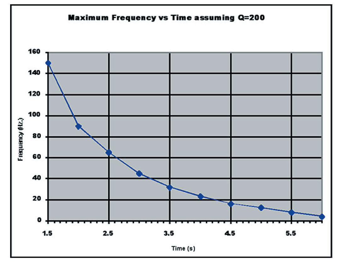
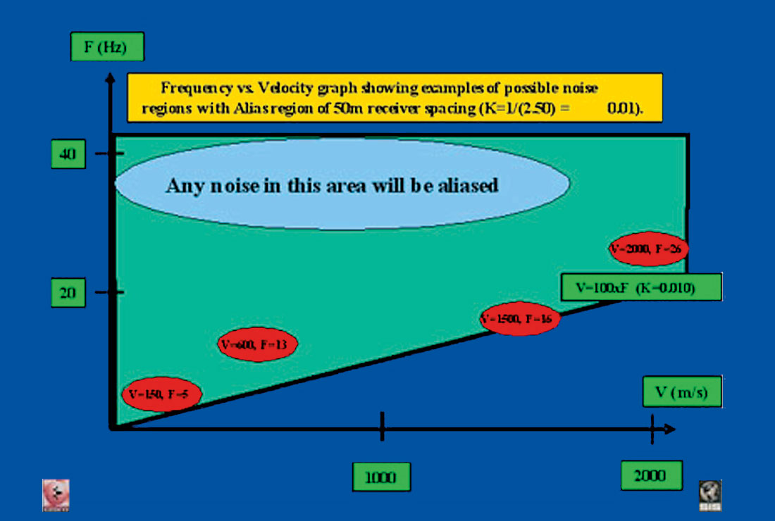
- From the estimated Q value, graphs (an example is shown in Figure 1) may be constructed showing available frequency vs time or depth. These are determined by taking into account spreading losses, transmission and reflection losses – and the inelastic attenuation (Q). Once a signal has fallen to 110dB below its near surface amplitude, it can be considered lost, since the recording system has a total dynamic range of only 138dB (signal is 5 bits or less = 30dB). Note that application of pre-amp gain (from 0 to 60dB can be used to “move” the 110dB recording range over the areas of interest (e.g. shallow horizon to target) – thus keeping good quantization levels over all horizons (reflectors) of interest.
- Using petrophysical information (e.g. cross-plots of acoustic impedance vs porosity), establish the criteria for detectability – which is the smallest change that we wish to see at the target level. For example a 5% change in porosity may show up on a seismic trace as an 8% change in acoustic impedance. If the seismic noise level is higher than this value, then we will not be able to detect the change. Hence we can establish the desired S/N.
- From the study of total attenuation (point 3 above), we can evaluate the attenuation of the detectability criteria – and hence the maximum frequency we will be able to see at the target. This may be less than Fmax (point 1 above). In such cases, there is no alternative but to accept this new (lower) Fmax – because the earth itself will prevent us from acquiring any higher frequencies at the target.
In a marine environment, the calculations are straightforward. The ambient noise level is usually well known (so many microbars of noise) and the source strength is also measured in similar units – so many bar-meters. Thus once the attenuation of the detectability criteria is known, this can be used to calculate the required source strength to keep the signal above the ambient noise level. On land the situation is not so simple and field tests are usually necessary to establish the desired source strength – which is the source that gives us Fmax from the target. - Now estimate the expected S/N of raw shot data. This can be done either directly on some typical test shots, or by dividing the S/N of a stack (or migrated stack) by the square root of the fold used to make the stack. Since Fold = (S/N of final migrated stack / S/N of raw data)2, then S/N raw = S/N migrated/Fold0.5.
Using the stack has the advantage that the S/N improvement due to processing is taken into account. Thus the subsequent calculations for the desired fold to achieve the desired S/N will be more realistic. When nothing is known about the area a useful rule of thumb is to require that the stack S/N=4. Any lower level on a final migrated stack will normally mean that the interpreter will have severe difficulties in identifying potential targets. Any higher level can be noted as an added bonus. - From the desired S/N (point 4 above) and the estimated S/N of the raw data (point 6 above), we determine the required fold of the survey.
- Next the required bin size is calculated.
Using Fmax (the required maximum frequency), we can estimate the horizontal and vertical resolution.
In the best case (maximum available migration aperture – and zero offset shot-receiver pairs), the resolution is approximately one quarter wavelength of the maximum frequency. This resolution is also equal to the bin size that will properly record the maximum frequency from a maximum dip angle (90 degrees).
Δx = Vrms / (4 . Fmax . sin(θmax)), where Δx = bin size
Thus the optimum bin size to use is given by Vrms / (4 . Fmax) – or one quarter of the wavelength of the maximum frequency.
In practice, this is often relaxed (a larger bin size is used), since it is really not practical (not to mention very expensive), to measure every dip with the maximum frequency. As an example, a velocity of 3000m/s and a frequency, Fmax of 60Hz leads to an optimum bin size of 12.5m – considerably less than is used on most land surveys today. A more typical calculation might say that we wish to measure up to an Fmax of 60Hz on dips of 30 degrees or less. This will relax the bin size needed to 25m.
The choice of maximum frequency is critical here. Fmax must be a practical choice – in other words the maximum frequency that can be reasonably well propagated from the surface source to the target – and back again to the surface receiver.
If Fmax is too high, then the consequent choice of bin size will be too small – and money will be wasted trying to properly record frequencies that are not available. Conversely if Fmax is too low, the bin size will be too large and high frequencies coming from dipping events will be aliased and will not contribute to the final migrated image. This second case is, in fact, standard operating procedure in many parts of the world. In other words, most surveys are undersampled!
Thus smaller bin sizes will normally improve the frequency content of dipping structures – but only to a certain limit which is that imposed by the earth as the total attenuation of the higher frequencies falls below the level where we can properly record them. - Next the minimum and maximum offsets (Xmin and Xmax) must be determined. These are normally calculated from muting functions used in processing – or automatic stretch mutes derived from velocities. A rule of thumb here is to use a stretch mute of the order of 25% - or 30% if long offsets are critical to success. The minimum offset corresponds to the shallowest target of interest – and the maximum offset to the deepest target of interest. These two values (Xmin and Xmax) will be used to determine approximate shot and receiver line spacings (equal to Xmin multiplied by the square root of 2 for single fold and equal line spacings) and the total dimensions of the recording patch.
- Migration Aperture:
Each shot creates a wavefield which travels into the subsurface and is reflected upwards to be recorded at the surface. Each trace must be recorded for enough time so that reflections of interest from sub-surface points are captured – regardless of the distance from source to subsurface point to receiver. And the survey itself should be spatially large enough so that all reflections of interest are captured within the recorded area (migration aperture). For complex areas, this step may require extensive 3D modeling.
Figure 2 shows an example of a model built for a complex sub-surface area. The section shown is an “in-line” display. The cross-lines showed the true 3-D nature of the model. Such models can be ray-traced to create synthetic 3D data volumes. The complex data resulting from such ray-tracing can be created with the correct times and amplitudes. This enables an investigator to observe the effects of processing – particularly PSDM from topography. By such means, the degree of illumination on any chosen target can be determined. In complex sub-surface areas, ray-tracing like this can establish the “visibility” or otherwise of a target for any specified 3D acquisition geometry.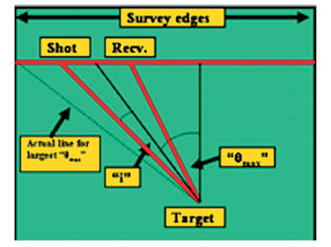
Figure 2.
The migration aperture (amount to add to the survey to properly record all dipping structures of interest at the edges) is normally calculated from a 3D “sheet” model of the target. Thus a colour display (where the colours are the values of the migration aperture), allows us to see how much to add on each side of the proposed survey. This gives the total area of shots and receivers. - Now various candidate geometries can be developed. The critical parameters of bin size (point 8 above) and fold (point 7 above) and Xmax (point 9 above) must not be changed. The shot and receiver intervals (SI and RI) are, of course, simply double the required bin size. Thus the only flexibility is to change the shot and receiver line intervals (SLI and RLI). But we must have Xmin2 = SLI2 + RLI2, (assuming that the layout of shot and receiver lines is orthogonal.). In most cases, it is not difficult to come up with a number of these “candidate” geometries – which all have the desired fold and bin size – and meet the requirements of Xmin and Xmax.
Typical variations that can be tried are small changes of line intervals (SLI and RLI), depending on whether shots or receivers are more expensive. Thus in heliportable surveys over mountainous terrain, shots are usually much more expensive than receivers – therefore we make SLI as big as possible to minimize the number of shots. In OBC surveys, receivers are much more expensive than shots (air-guns). Therefore we make RLI as big as possible.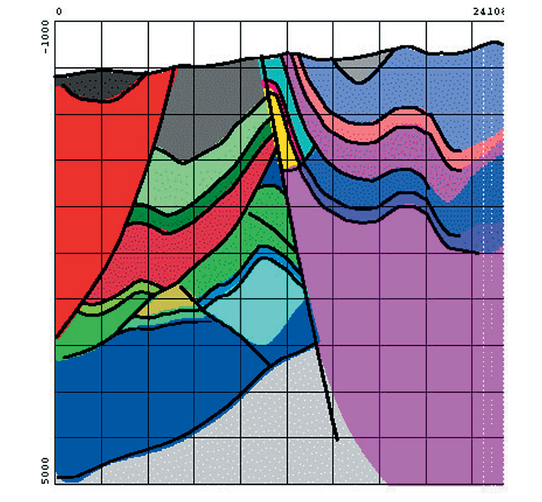
Figure 3.
In all cases of orthogonal geometries, it is not wise to stray too far from shot and receiver symmetry. As the lack of symmetry increases, the shape of the migration response wavelet will change – leading to undesired differences in resolution along two orthogonal directions.
Many surveys use different shot and receiver group intervals. Such practices will cause different resolutions in the shot line and receiver line directions. Thus a true 3D structure will not be properly imaged in all directions. Interpolation will NOT correct these problems. What has not been measured in the field (small spatial wavelengths in both directions) cannot be recovered by processing techniques. - The candidate geometries can each be tested for their response to various types of noise – linear shot noise, back-scattered noise, multiples and so forth. They can also be tested for their robustness when small moves of shot lines and receiver lines are made to get around obstacles. The “winning” geometry will be the one that does the best job of attenuating such noise. Naturally because all of the candidate geometries were chosen to have the optimum bin size, required fold etc. the “winner” will also have the optimum imaging properties.
Aliasing of certain noise trains can be a big problem. Thus at this stage shot and geophone arrays can be added to the design problem to examine their effect on expected noise trains. Crossplots of frequency vs. velocity are most useful here – noise trains which have a certain frequency and velocity become points in these plots. Shot and receiver intervals (SI and RI) become radial lines from the origin at a slope corresponding to the spacing. “Islands” of noise above the line represent aliased noise – and noise below the line re p resent properly sampled noise which could be removed by any of the standard processing techniques – FK, Tau-P etc.. - Acquisition logistics and costs may now be estimated for the “winning” geometry. Depending on the result (e.g. over or under budget) small changes may be made. If large changes are needed, the usual first casualty is Fmax. Thus dropping our expectations for high frequencies will lead to larger bins which will lead to a cheaper survey. Another possible casualty is the desired S/N – or in other words – using lower fold.
- It is often the case that there will be unanswered questions after the design is finished. Thus field tests can often resolve these final problems. For example, dynamite shot costs depend critically on the depths of the shot holes. Only a series of field tests can properly answer the question of the optimum shot hole depth – and charge size.
Thus field tests conducted before the main survey can be used to answer such things as:
Source choice (depth of hole/charge size, vibrator parameters – ground force, sweep frequencies, arrays etc.)
Receiver choice (buried or not – geophone type, etc.)
Arrays – both shot and receiver – to suppress shot-generated surface noise.
Recording Gain – to optimize sampling of frequencies at target levels.
Summary
The primary goal of any 3D is to achieve the desired frequency and S/N at the target!
To ensure the best image, the best sampling method that can be used to recreate the various spatial wavelengths in X, Y and Z must be chosen. G. Vermeer has written the book on this approach (3D seismic survey design, SEG, 2002) and it involves symmetric sampling – whatever is done to shots must also be done for receivers.
Noise attenuation can be just as important as signal. It is worth remembering that if the CMP stack for one geometry attenuates the noise by 6dB when compared to the CMP stack for another geometry, the fold has been effectively quadrupled. This can have a dramatic effect on the budget!
Some of the best geometries for noise attenuation are wide azimuth slanted geometries with 18.435 degrees often emerging as the winning angle. The small departure from orthogonal (18 degrees instead of zero) has only a very small effect on the imaging properties. Wide azimuth orthogonal surveys where the shot line interval is not quite equal to the receiver interval can be even more successful than slanted lines in attenuating noise.
For noise reduction (both linear, backscatter and multiples), many authors have noted that wide azimuth surveys will be better than narrow – simply because there is a larger percentage of long offsets in a wide survey.
Budget? Be prepared to spend some money! There is nothing as expensive as a 3D that cannot be interpreted!
Q.2: Do wide azimuth surveys exist?
Yes, such geometries are feasible and yes, they are being used.
Many land 3Ds are now shot using a square recording patch – with orthogonal shot and receiver lines. However as the shot and receiver line intervals are usually much greater than the shot and receiver group intervals, the offset distribution is somewhat irregular – although it does repeat from “box” to “box” (area between two shot lines and two receiver lines).
To find true well sampled 3Ds with uniform offset and azimuth distribution we can look at two examples in the marine world.
The first example comes from the world of OBC (Ocean bottom cable). There are two main OBC geometries being used today – “swath” and “patch”.
The “swath” geometry lays out two parallel receiver cables - perhaps as much as 12 km in length and typically 400m or so apart. A gun boat sails down between the two receiver lines – and parallel to them – taking shots frequently (every 25m) with perhaps 50m from one sail line (shot line) to the next.
This is exactly equivalent to a marine anti-parallel geometry with two streamers and multiple sources. Here the offset distribution is more or less uniform. The azimuth distribution is however confined to a small “cone” between the two receiver cables.
The “patch” geometry is more interesting. Here the two cables are again laid out – perhaps some 300m apart (with receivers spaced every 50m down each cable. This time, the gun boat sails orthogonal to the cables starting some distance away from the two cables (perhaps as much as 6km) and sailing across them to as much as 6km on the other side – with shots fired every 50m. Then the gun boat moves to a parallel shot line (possibly 150m away) and shoots this second shot line (again maybe 12km long with shots every 50m). The shot lines are repeated until an entire area around the two receiver cables has been acquired – at which point the cables may be moved to a new position and the exercise repeated in an overlapping fashion.
Such a survey is very close to a wide azimuth, wide offset geometry – with all the normal desired azimuths and offsets. In the author’s experience, several such OBC’s have been acquired in the past 10 years – all over the world. The example above (300m receiver line interval and 150m shot line interval with staggered shots from one line to the next) was shot in the Middle East some 3 years ago – and the resulting data was the best that had ever been seen in that area.
The second example of a uniform offset wide azimuth survey comes from the world of permanent receiver geometry (for time lapse – or 4D- surveys). Here the receiver stations are spaced approximately every 300m along each receiver line with 300m between lines – thus a grid of receivers every 300m on the sea bottom. The airgun boat (source vessel) sails shot lines which are 50m apart – and pops every 50m – thus forming a continuous grid of shots every 50m on the surface. Again such a geometry (usually called an areal geometry) does not quite have a uniform azimuth/uniform offset distribution, but it is very close to the fully sampled 3D geometry.
Such geometries are possible due to very cheap sources (in these cases air guns). Recent innovations in land sources (weight drop methods) mean that it should be possible to create such geometries on land - at similar costs. Finally shot-receiver reciprocity means that cheap receivers can also be used to make such geometries.


Share This Column