What Should Multicomponent Near-Surface Corrections Look Like in a World of Waveforms?: A raypath-consistent solution for converted-wave processing

Removal of near-surface effects from elastic data, particularly converted waves, is a well-known and difficult problem, whose difficulty only increases on the backdrop of the trend in our field towards treating seismic wiggles as full waveforms. If we want to eventually apply some type of full waveform inversion or fitting, or if at any rate we want to reserve the ability to do so, we face the question: to what degree are data still understandable as measurements of a wave field after traditional statics have been applied?

We could remove this worry by developing methods for near-surface correction which themselves are consistent with the wave view of seismic data, but are “full waveform-consistent statics” possible? We think so, in fact one of us (Henley, 2012) has argued along these lines. In this paper we will not go quite that far, but will be satisfied to take a significant step in the direction of waveform consistency. The approach we discuss and exemplify will be, if not waveform-consistent, then at least raypath-consistent. The purpose of this paper is to summarize the approach, which is described in more technical detail elsewhere (Cova et al., 2016a,b), focusing on results over theory.

Changes in the velocity and thickness of near-surface sediments introduce delays and other variability in seismic data, which greatly increase the complexity of the data but not their information content, relative to deeper geological features. As a result, the actual structure and alignment of the subsurface reflections is distorted to the detriment of the stacking power and resolution of the seismic events. In the case of converted-wave data, the very low velocities of shear waves in the near-surface aggravate the problem, and render some of the simplifications allowable when solving P-wave statics unsuitable. Since the velocity of S-waves is not significantly affected by the presence of fluids in the pores, the velocity structure of the near-surface “seen” by S-waves may differ from that controlling P-wave propagation. These attributes of S-wave statics lead to a very complex overall problem (Stewart et al., 2002).

Conventionally, P- and S-wave near-surface corrections are addressed by assuming surface-consistency. This is the origin of the term “statics”, i.e., that a single constant time shift is computed and applied per trace to remove the near-surface effect. The largest assumption behind this idea is that a significant velocity contrast exists between the low velocity sediments in the near-surface and the underlying geology. By Snell’s Law, such large contrasts result in near-vertical raypaths through the near-surface layers, regardless of the obliquity with which the ray was incident from below on the near-surface.

S-wave velocity variations in the near-surface defy these assumptions to a degree that can seriously harm the statics solutions. The actual raypaths of the waves are too different from the assumed vertical raypath models for the corrections to be accurate. Velocities are usually smoother for S-waves than for P-waves (Yilmaz, 2015), therefore, the S-wave velocity contrast at the base of the near-surface may not be large enough to produce vertical rays. Also, the wider incidence angles needed to observe strong converted S-wave energy threatens this assumption.

Henley (2012) introduced an alternative approach, based on the concepts of interferometry, in which raypath consistency is adhered to. That is, in which ray obliquity is permitted. The approach also benefits from being data driven, such that no velocity model for the near-surface is needed. The approach has been successfully demonstrated in both P- and S-wave statics applications. The problem of raypath-dependent statics was addressed by using the radial-trace (RT) transform to transform the data to a domain where amplitudes are a function of raypath angle. The main weakness of the approach is that the RT transform remaps amplitudes assuming an underlying constant velocity model. Put another way, the raypath consistency we seek is only provided if the medium has no spatial variations.

The work we will summarize in this paper involves using the τ-p transform as a more complete way of obtaining raypath consistency. This movement of the data to the ray parameter domain accommodates vertical variations of velocity. A key issue addressed in the work is the non-stationarity of the problem, i.e., the tendency for the correct static shift to not be static is considered. An important aspect of the work is that near-surface effects are extracted from the reflected data. Therefore, no first break analysis or refraction data are needed.

Our metric for determining the success of this approach is the event stacking power and coherence, in particular, the degree to which stacking power is sustained for both shallow and deep events. We will show how accounting for the non-stationary character of the near-surface effects provides stacking power improvements for both shallow and deep events simultaneously.

The Idea of Raypath Consistency

Data analysis in the ray parameter domain

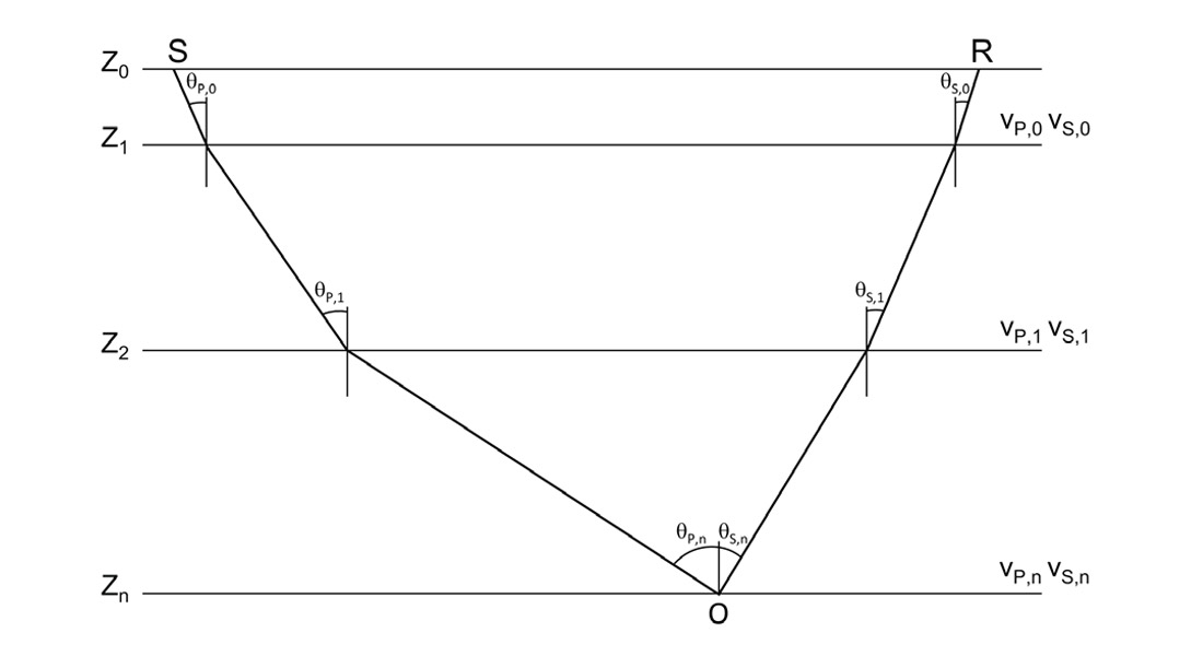
The ray parameter “p” as determined from data recorded on surface arrays is related to the angle at which the wavefield emerges at the surface (Tatham, 1989). This makes the ray parameter domain a good environment for characterizing near-surface effects. According to Snell’s law the ray parameter p is constant when the wavefield propagates in a horizontally stratified medium. The conservation of the horizontal slowness applies also to converted waves. For the PS raypath depicted in Figure 1 the relation

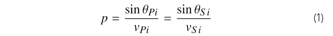
holds, where v_Pi and v_Si are the P- and the S-wave velocities in the i-th layer and θ_Pi and θ_Si are the P- and S-wave propagation angles. This expression allows the full raypath of a converted-wave to be described via a single ray parameter value, in spite of the fact that the P- and S-wave legs involve different wave velocities.

Data are moved to the ray parameter domain through the application of the “slant-stack” or τ-p transform (Stoffa, 1989). This involves stacking data along straight lines within a given range of slopes (p) and intercept times (τ).

Because seismic reflection data exhibit hyperbolic moveout, the τ-p transform amounts to scanning for all the possible tangents that contribute to such hyperbolas. The “scanning” nature of the transform relieves it of the need for any a priori knowledge of the velocity model of the subsurface.

Carrying out raypath-consistent near-surface corrections

In a layered medium, the intercept time τ represents the aggregate vertical slowness-thickness product (Diebold and Stoffa, 1981):

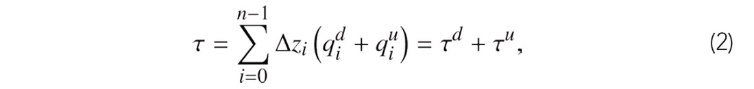
where q_i is the vertical slowness q_i = cos(θ_i)/v_i in the i-th layer, and Δz_i is the layer thickness Δz_i = z_i+1 − z_i. The superscripts ^d and ^u label the down-going and up-going legs of the raypath in Figure 1, respectively. For converted waves, the down-going vertical slowness is determined by the P-wave velocities, and the up-going vertical slowness by the S-wave velocities.

To better understand the effect of the near-surface on the receiver side, let us next isolate and expand the up-going contribution to the intercept time τ, which is

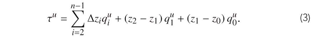
If we assume that the measurement surface z₀ is at depth z₀ = 0 m, we can rearrange the terms in a convenient way, finding:

Now consider this expression term by term. The first term is the total contribution to the vertical travel time from the up-going wave generated at the conversion point and traveling up to the base of the second layer. The second term is the rest: the contribution due to propagation from the base of the second layer up to the surface. This occurs with velocity v₁ and raypath angle θ₁, as if the layer with velocity v₀ were not present in the model. The effect of the near-surface layer with velocity v₀ and thickness z₁ appears only in the last term. Therefore, to remove the near-surface effect we isolate and subtract this term from the total intercept time. The receiver-side near-surface correction can then be written as

The correction in Equation 5 works in an interesting way. The τ contribution of the near-surface layer (z₁q₀) is removed, then replaced by the τ contribution obtained with the ray parameter controlling the propagation in medium 1. Therefore, near-surface corrections are obtained by first replacing the near-surface layer velocity with the velocity of the lower medium (i.e., a replacement medium), then by extending the raypath parameters of the lower medium up to the surface. This is what we mean by a “raypath-consistent” correction.

The delays introduced to a seismic record by a horizontally layered medium are constant for a constant p value. This is seen by considering how the vertical slowness q is related to the ray parameter value:

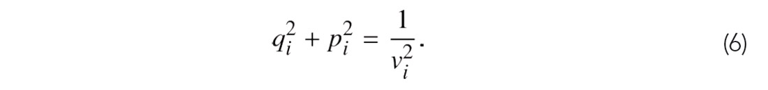
Because the ray parameter is a constant in a horizontally layered medium, Equation 6 shows that if p is fixed, the delays introduced by the near-surface, which are a mixture of its thickness and the vertical wavenumber, must be fixed for a fixed p-value.

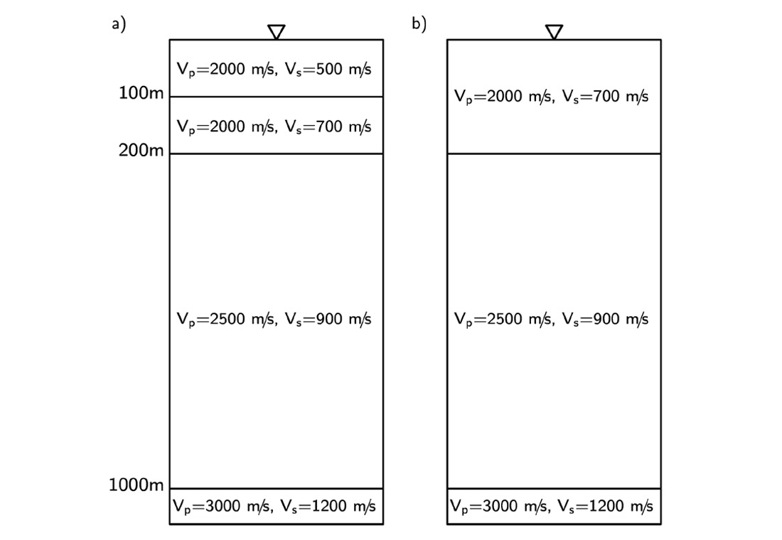
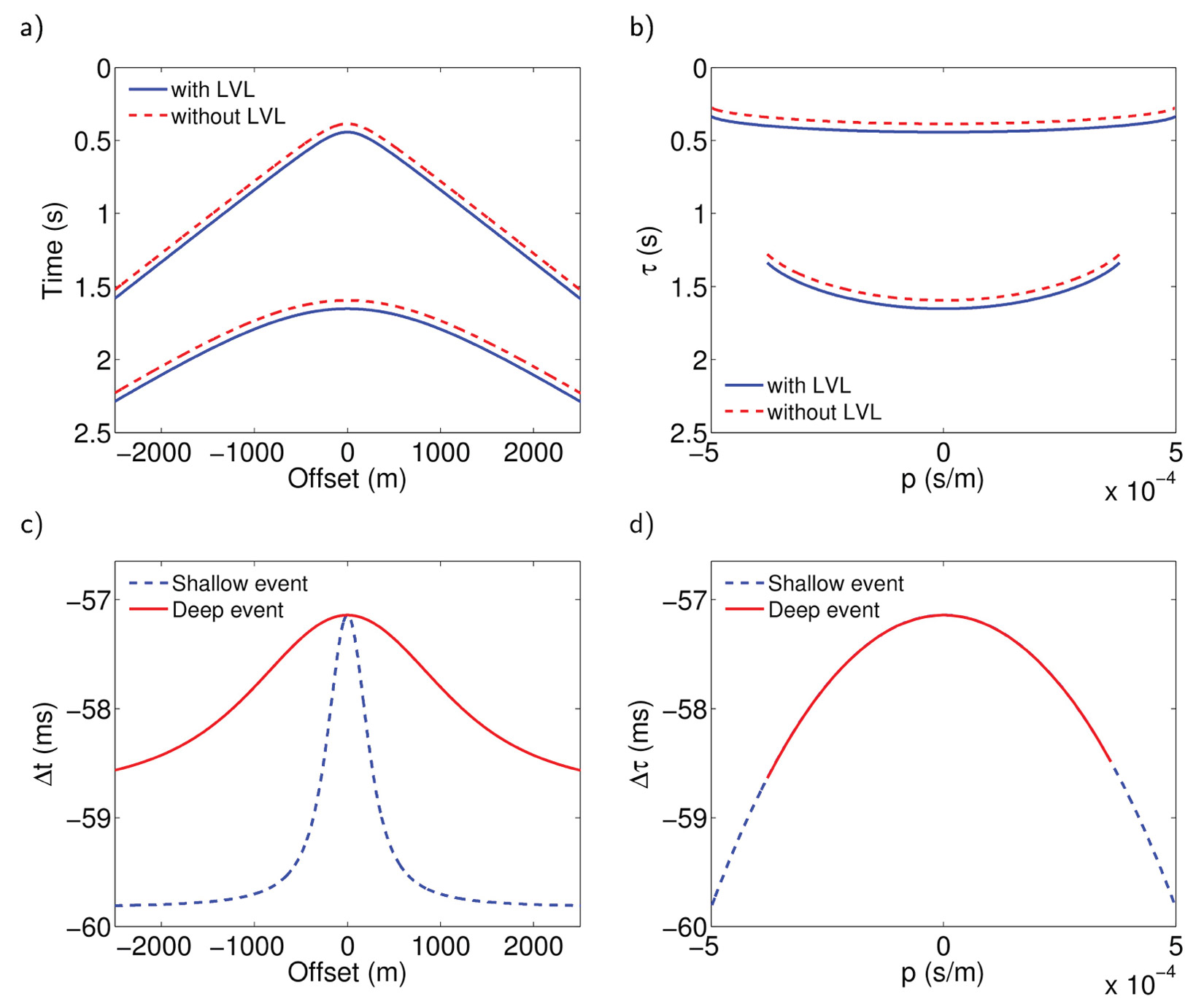
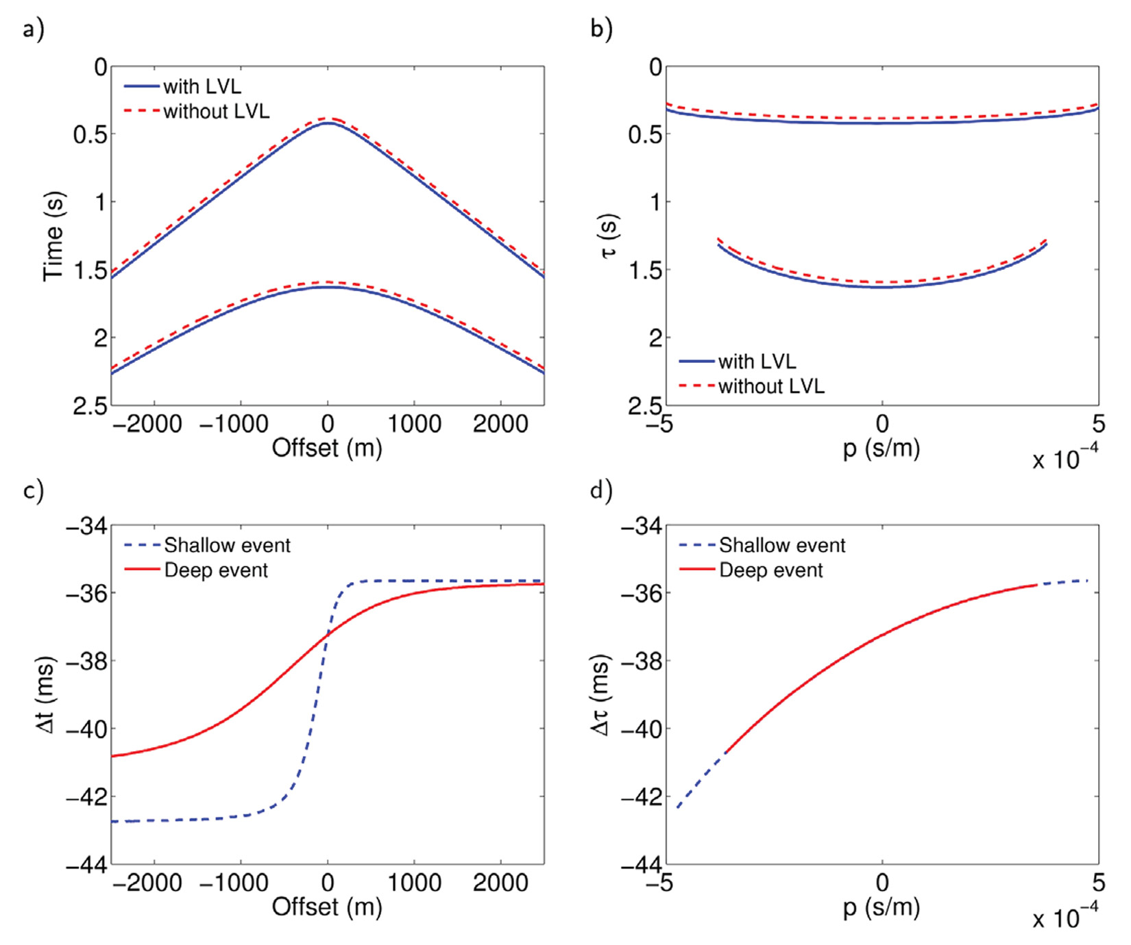
What benefits should we expect to see by taking advantage of all this, and going the ‘raypath consistent’ route? A big one has to do with nonstationarity – the tendency for statics not to be static. Let us illustrate how nonstationarity enters by using a numerical example created with PS-raytracing over the velocity models illustrated in Figure 2. A situation in which source-side near-surface corrections have already been applied is simulated by including no P-wave velocity contrast in the near-surface layer. Figure 2a depicts a model with a low S-wave velocity layer in the near-surface. Removing the near-surface layer and replacing it with the velocity of the medium underneath results in the velocity model represented in Figure 2b. The resulting travel times are plotted in time-offset (Figure 3a) and τ-p (Figure 3b) coordinates.

Next, we subtract the travel times calculated above with and without near-surface effects for each event. These differences are illustrated in Figure 3c and Figure 3d.

From Figure 3c, it is evident that the corrections needed to remove the effect of the near-surface in the time-offset domain are non-stationary. The magnitude of the corrections not only changes with offset but also depends on the depth of the event. This is because the correction depends on the raypath. For a fixed offset, energy arriving from deep interfaces will arrive following raypaths with angles closer to the vertical, whereas those from shallow interfaces will enter the near-surface with wider raypath angles. For this reason, the shallow events will need greater degrees of correction than deeper events.

Figure 3d confirms that in the τ-p domain, the correction needed to remove the near-surface effect is the same for both events. For a fixed ray parameter value, a constant τ correction will suffice to remove the delays caused by the near-surface on both events.

Dipping near-surface layer

Equation 2 holds for dipping interfaces (Diebold and Stoffa, 1981), however, the ray parameter value p is no longer constant, and its computation requires us to consider the dip of each interface.

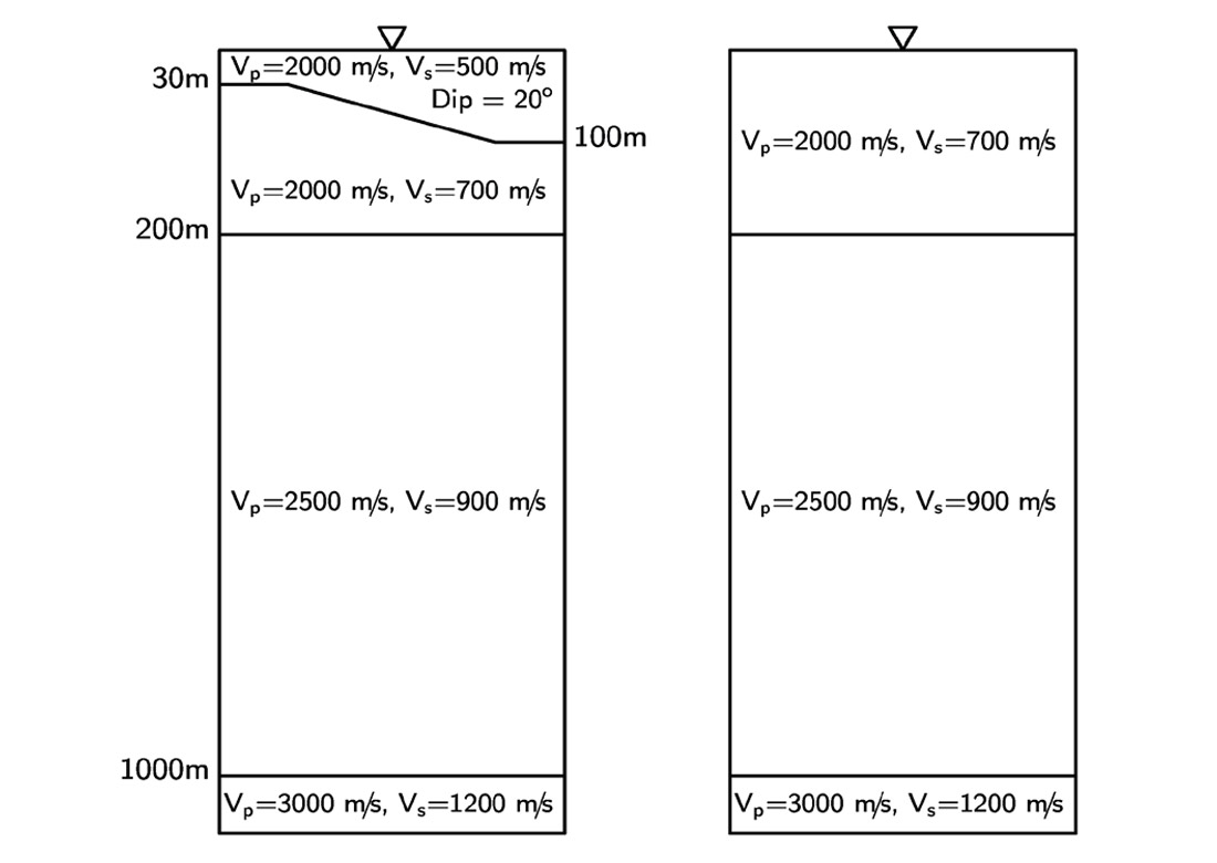
To see how dipping near-surface interfaces affect corrections, the model in Figure 4 was used to ray-trace converted-wave travel times. As before, these are compared with the ones obtained from a model with no low velocity layer in the near-surface, in both time-offset (Figure 5a) and τ-p (Figure 5b) domains. The travel time differences for each event are plotted in Figure 5c and 5d. We find that the raypath-dependency of the correction has been increased. Since the vertical thickness beneath the receiver location is 65 m, the magnitude of the corrections is smaller than in Figure 3. However, the range of the corrections is now larger, and is indeed asymmetric. For the shallow event, negative offsets will need a correction of about 43 ms while positive offsets will require a correction of 36 ms. This confirms again the strong non-stationarity of the problem as analyzed in the time-offset domain. However, the results in the τ-p domain still exhibit robust stationarity.

Raypath-consistent Corrections in the Field

The processing flow used to remove near-surface effects from field data is summarized in Figure 6. It is a modified version of the workflow introduced by Henley (2012), in which near-surface effects are captured and removed by using interferometric principles. Here, input receiver gathers are transformed to the τ-p domain and gathered into common-ray parameter panels. A set of pilot traces which represent a model of the data without near-surface effects is then computed. The pilot traces are obtained by enforcing continuity on the seismic events after sorting the data into common-ray parameter panels.

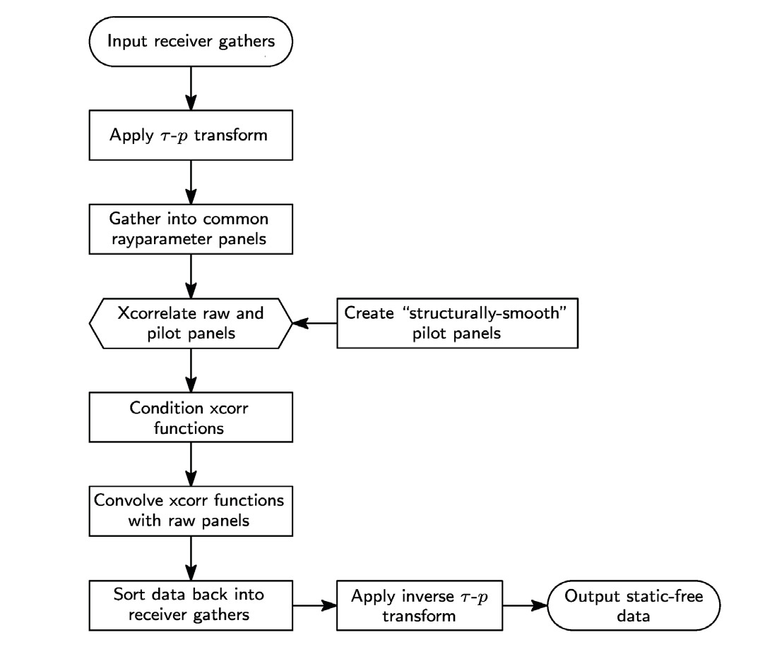
The set of cross-correlation functions output from these steps must next be conditioned to be used as matching filters. Whitening the spectrum of these functions is also needed so that the original amplitude spectrum of the data is preserved. Hanning weighting (Henley, 2012) is then used to attenuate or suppress any spurious energy captured during the cross-correlation operation, especially at unrealistically large time lags. The resulting conditioned functions are then primed to remove, through correlation, the near-surface signatures.

Hussar dataset example

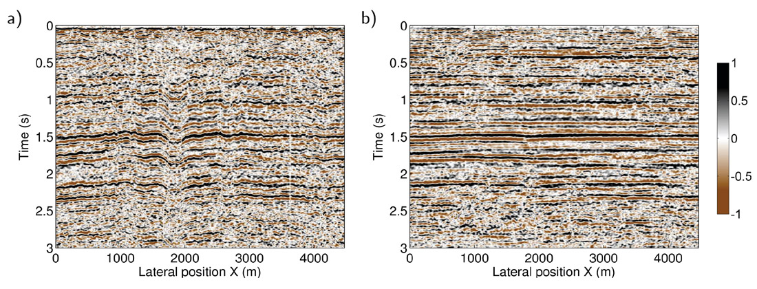
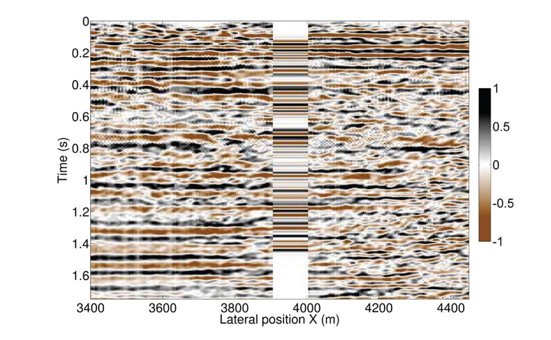
In 2011, the Consortium for Research in Elastic Waves Exploration Seismology (CREWES), in collaboration with several companies, carried out a seismic experiment in the Hussar area in Southern Alberta (Margrave et al., 2012). Although originally designed to investigate broad-band inversion schemes, the preliminary processing of the horizontal components revealed the presence of important nearsurface effects. Figure 8a shows a common-receiver stack of the radial component data after surface wave removal and source static corrections. Notice how the events between the x-locations 1500 m and 2500 m are pulled down due to low velocities in the near-surface. In this region, we can also observe how the near-surface causes the continuity of the events to be interrupted by jumps between consecutive receiver stations.

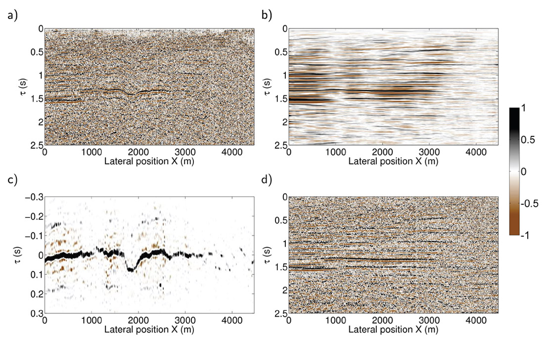
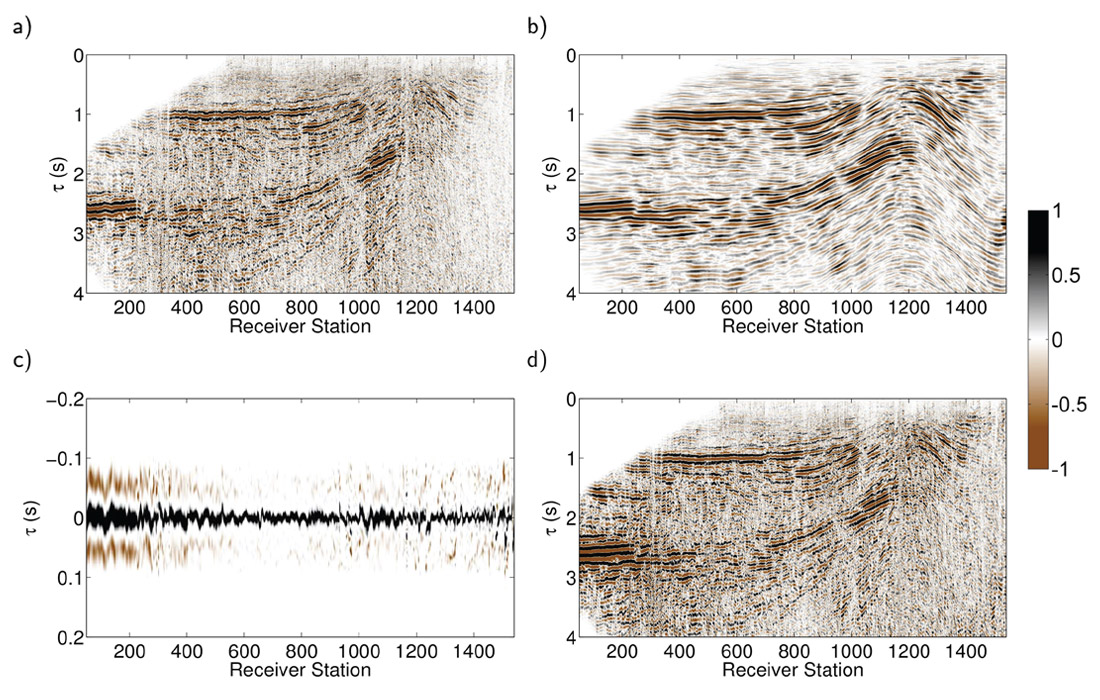
Figure 7 illustrates each stage of the processing flow in Figure 6. Figure 7a represents one of the common-ray parameter panels obtained after transforming common-receiver gathers to the τ-p domain. A pilot panel (Figure 7b) is then computed by applying trim statics and a moving average process to artificially remove the shifts between traces, and enhance the continuity of the events. The cross-correlation between the input panel and the pilot traces is plotted in Figure 7c. Notice that the pattern of the apparent lags of the cross-correlation traces has captured the event deformation present in the input panel. Spectral whitening and Hanning weights have been applied to these traces to increase the bandwidth and suppress energy at very large lags, respectively. The near-surface corrections are then applied by convolving the input traces with the conditioned set of cross-correlation functions (Figure 7c). Notice that the deformation present in the input panel between the x-coordinates 1500 m and 2500 m has been removed. Moreover, the continuity and coherence of the events all along the section have been significantly improved, probably because local phase and event arrival uncertainties were removed by the deconvolution operations.

This process is applied over all the common ray parameter panels available. Following this, an inverse τ-p transform returns the data back to the time-offset domain.

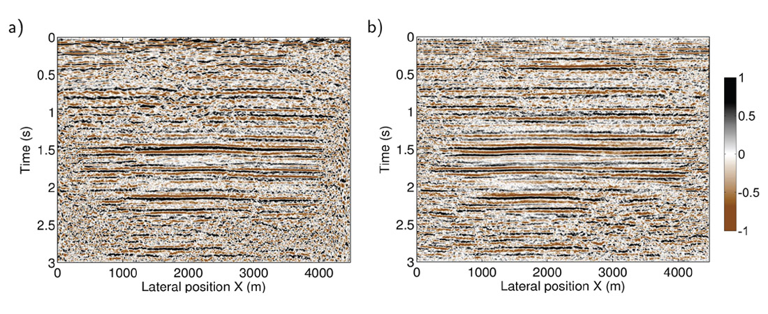
The common-receiver stack after near-surface corrections (Figure 8b) shows very significant improvements in the alignment and stacking power of the events in the section. This is especially true at times less than 1 s where almost no coherent energy was initially recognizable. The same observations can be made on the common-conversion-point (CCP) stack plotted in Figure 9b. A CCP stack obtained by using a more conventional surface-consistent solution is displayed in Figure 9a for comparison purposes. Although on both sections the coherency of the event around 1.5 s has been improved and the deformation removed, the raypath-consistent solution displays superior results at shallow times (< 1 s).

Dipole sonic data from a well located around the x-coordinate 3950 m was used to compute a synthetic converted-wave seismogram. The well tie displayed in Figure 10 confirms that the events in the shallow part of the sections are correlated with rock property changes recorded in the well logs.

Sinopec dataset example

A 2D-3C seismic line provided by Sinopec was processed to test raypath-consistent near-surface corrections in the presence of smooth structures. The processing flow used on this dataset was introduced in Figure 6.

In the processing of data from structurally complex areas, computing pilot traces may require additional steps. In particular, the structural features present in the data must be preserved at all times. Therefore, forcing coherency on the seismic events while creating pilot trace panels must be handled carefully. To compute the pilot traces in Figure 11b, the data were flattened to a horizon following the structural trend seen in Figure 11a. After removing the structural trend, trim statics and lateral trace averaging were used to force continuity on the events. For the lateral trace averaging, Gaussian weights were applied to the traces within a window before averaging. In this way, we intend to localize the averaging process around each fixed receiver location while still using reasonably wide windows (approximately 50 traces).

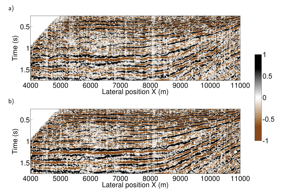
After all the ray parameter panels were corrected, the data were sorted back into receiver gathers and an inverse τ-p transformation was performed. Figure 12 displays CCP stacks before and after near-surface corrections, zoomed around receiver stations 400 to 1100. Notice that all events exhibit better coherency after correction. Moreover, in Figure 12b we observe that the seismic resolution has been improved on the data above 0.8 s. Since shallow events covered a wider range of reflection angles, they benefited most from removal of near-surface effects in this raypath-consistent framework.

Conclusions

We have demonstrated a technique for determining and applying receiver-side surface corrections to converted-wave seismic data. Raypath-consistent near-surface corrections do not require first breaks or a starting model for near-surface velocity structure. The method utilizes the new concept of raypath consistency to accommodate the inherent nonstationarity of surface corrections for shear waves. Through the use of the interferometric operations of cross-correlation and match filtering, the method also attempts to enforce wavefront consistency by removing local wavefront arrival uncertainty and phase differences.

The ability of raypath-consistent corrections to accommodate near-surface effects for shallow and deep events simultaneously is one of the most important features of this approach. In the processing of deep converted-wave data only, the assumption of vertical raypath angles may be sufficient for the use of a surface-consistent approach. However, the very low velocity of S-waves and the ability of shallow events to reach wide reflection angles requires a raypath-dependent framework. The methodology shown in this study demonstrates how this can be achieved even when the geology of the area presents some structural complexity.

Acknowledgements

The authors would like to thank Sinopec for providing the data and permission to publish these results. This work was funded by CREWES industrial sponsors and NSERC (Natural Science and Engineering Research Council of Canada) through the grant CRDPJ 461179-13.