Well Tie Methodology: A Very Often Overlooked Critical Step in Seismic Interpretation and Inversion

Abstract

Well tie to seismic is one of the first and basic steps in the process of seismic interpretation and seismic characterization. The process very often is overlooked, and the consequences are not comprehended. In this article, we will explore the basics of the well tie to seismic, starting with some basic seismic acquisition and processing concepts, definition and type of wavelets and a case study that will show the impact of using a wrong estimation of the time-depth relationship (obtained from the well tie process) in future workflows such as seismic inversion. We will explore the effect on using different wavelets in a simple simultaneous seismic inversion, and the consequences it may represent when estimating elastic and geomechanical properties.

Introduction

It is well known that well tie to seismic is a critical step towards the characterization of reservoirs using seismic data. Nonetheless, this process is frequently overlooked by seismic interpreters and QI geophysicists. There can be several reasons for that, but we believe that a qualitative approach is often to blame when the results are not those that we expect. Understanding the real characteristics of the wavelets (amplitude, phase, and frequency) and their variations with each other (e.g. amplitude and frequency and phase and frequency) is paramount to perform an optimal well tie. We agree that a quantitative approach is needed (not just a visual comparison between synthetics and seismic data, assuming at the same time knowledge of the wavelet being analyzed) when doing well ties. It is also important to note that to have a good well tie, a proper wavelet estimation should be performed.

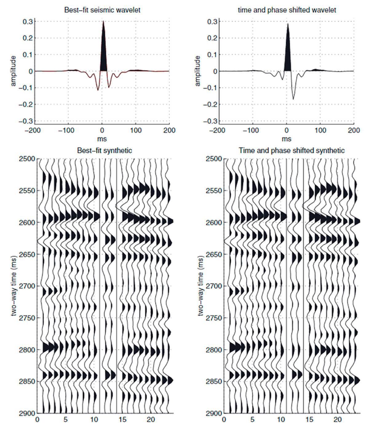
Several authors have shown the effect of assuming wavelet characteristics when performing well ties. Roy White, 2005, showed how ‘well’ two different synthetic seismograms, obtained from two distinctive wavelets, can ‘match’ visually the seismic data.

Figure 1 shows how two distinctive wavelets can result in a very comparable (qualitatively speaking) seismic-to-synthetic match. Later in this article, we will show how using the wrong wavelet can impact the elastic properties estimated from seismic inversion.

When performing well to seismic ties we want to achieve several things:

• Satisfy ourselves that there is a reasonable match between synthetic and seismic data at the objective level, without which inversion will not be useful.
• Establish the time-depth relation that will be needed for building the starting model.
• Determine the offset (or angle) - dependent wavelets that are needed as input to the inversion.

In general, we should establish the well ties at the start of the inversion preparations, but seismic data conditioning will change the time-depth relations and the wavelets, so the well ties should be repeated on the final conditioned seismic.

We will explain in some detail the Roy-White methodology (White, 1980) as a way to quantify how good a well tie is (and hence, demonstrate improvement after log editing or seismic conditioning) and to put error bars on the seismic wavelet spectrum (so we can see whether the wavelet is well determined).

Seismic basics

We need to understand the principles of polarity, wavelet’s phase, amplitude and frequency, and amplitude and frequency attenuation, including phase change with offset/angle, in order to perform a proper well tie.

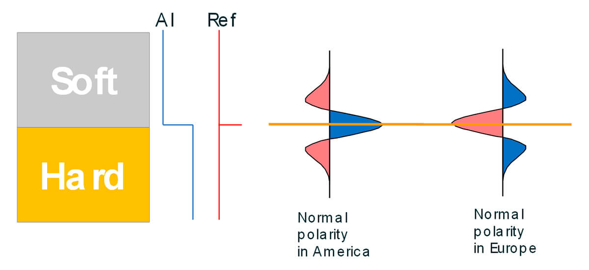
In order to perform a proper well tie, it is important to know the polarity of our seismic data. This is a process that in general takes virtually no time to analyze. Generally speaking, the interpreter with some geological knowledge can identify geological layers where densities can be higher than the surrounded layers (like limestone or dolomites for example, or shales between sands). In this case, we expect an increase in impedance and a peak in the seismic data expected. For marine data, we usually look at the water bottom interface. If we observe a peak on the water bottom (positive values of amplitudes), we have normal polarity in America. On the other hand, if we observe a trough on the water bottom, we are in normal polarity in Europe (Figure 2).

Europe (Figure 2). As we know, the seismic wavelets are characterized by their amplitude, phase, and frequency spectra. Let’s review these concepts very briefly.

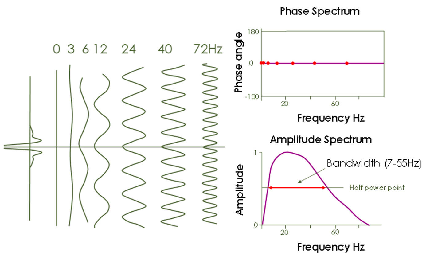
Phase describes the relative timing of these various frequency components. We analyze the phase of a wavelet in a Phase Spectrum plot. Frequency describes how many oscillations per second (Hertz) can be estimated in a wavelet. The amplitude spectrum describes the amplitude of the different frequency components of the wavelet. In other words, an amplitude spectrum shows the amount of ‘energy’ within each frequency component that constitutes the whole wavelet. In Figure 3, we describe Phase, Amplitude and Phase Spectrum plots for a zero phase wavelet (where there is no time lag between the different frequency components that make up the wavelet).

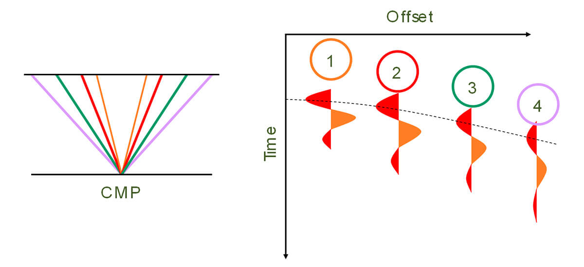
The frequency and amplitude of seismic energy attenuate with traveled distance; therefore, wavelets that penetrate deeper reservoirs will travel longer and will have less amplitude and frequency content (also known as bandwidth) than wavelets traveling through shallower targets. At shallower targets the effect of attenuation can be observed at large offsets. Figure 4 shows an example of a Common-Mid Point (CMP) reflection where the near trace (1) has a higher amplitude and shows higher frequency content than the far trace (4). The low-frequency content of the far traces at shallower targets is even more affected when we perform Normal-Move Out (NMO) to make the reflection hyperbola flat before stacking. This process will ‘stretch’ the far trace even more, decreasing its real frequency content. In seismic processing, these traces are typically muted to avoid interference of artificially low-frequency content due to NMO stretching.

Well ties and wavelets

We want to achieve several things with the well ties:

• Satisfy ourselves that there is a reasonable match between synthetic and seismic data at the objective level, without which inversion will not be useful.
• Establish the time-depth relationship that will be needed for building the starting model needed for seismic inversion. Either for building the low-frequency model needed for simultaneous seismic inversion or for QC seismic inversion techniques that do not need such a low-frequency model (e.g., facies-based inversion).
• Determine the offset (or angle) dependent wavelets that are needed as input to the seismic inversion.

In general, we should establish the well ties at the start of the inversion preparations, but seismic data conditioning will change the time-depth relations and the wavelets, so the well ties should be repeated on the final conditioned seismic.

A quantitative approach for the well tie: the Roy White methodology in practice

The Roy White methodology (White 1980) allows us to quantify how good a well tie is, and hence, demonstrate improvement after log editing or seismic conditioning. It allows us to analyze error bars on the seismic wavelet spectrum so we can see whether the wavelet is well determined.

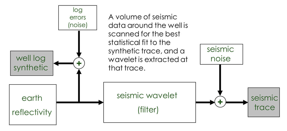
The Roy White method is essentially a coherence matching technique. The workflow can be summarized as follows:

1. From well log data we estimate the earth reflectivity, albeit with associated noise.
2. A volume of seismic data around the well is scanned for the best statistical fit to the synthetic trace, and a wavelet is estimated at that trace.
3. The filter providing the best match between the earth reflectivity and the seismic is our best estimate of the original seismic wavelet.

In an inversion, we are attempting to remove this wavelet from the seismic, so clearly, it’s vital to know what it looks like. Figure 5 shows the schematized Roy White methodology.

There are various things to consider when tying a well and estimating wavelets. The first is the wavelet length or L. Then there is the time window, T, over which the estimation will be performed.

Roy White defined two important concepts useful to quantify the quality of a well tie: the goodness of fit, and the wavelet accuracy. Maximizing these two measures should deliver the best wavelet, with the smallest error bars.

The goodness of fit measurement is called PEP, the proportion of energy predicted from the synthetic. Numerically, it’s approximately the square of the cross-correlation, and a value greater than 0.7 is considered good.

Goodness of fit is not a measure of the accuracy of the wavelet. The cross-correlation increases with increase in wavelet length, but the longer the wavelet is, the more chance that noise is also being matched.

If a value of one is achieved, it implies a perfect match between the seismic and the synthetic, using the estimated wavelet (i.e., the residual is zero).

The goodness of fit is defined by equation [1]:

The maximum PEP value is not necessarily found at the well location or along a composite trace along the well trajectory. In practice, a seismic cube is scanned around the well location in order to find a maximum PEP. This approach is preferable since positioning of seismic energy during migration carries uncertainty, well positioning itself may be uncertain, and lateral stability of the estimation may be better understood with PEP maps.

The wavelet accuracy is given by NMSE, the normal mean squared error, that is calculated using equation [2]:

Where L is the wavelet length and T is the length of the time window from which the wavelet is estimated. A good well tie has NMSE less than 0.2.

The window T we choose is a function of the frequency content of the seismic or the bandwidth. The higher the bandwidth, the smaller the time window.

The wavelet length is then simply calculated from the time window. Usually, L is a value between a 1/3 and a 1/7 of the time windows used.

The relationship between the Goodness of Fit and Wavelet Estimation error as a function of the ratio 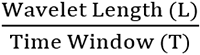can be seen in Figure 6.

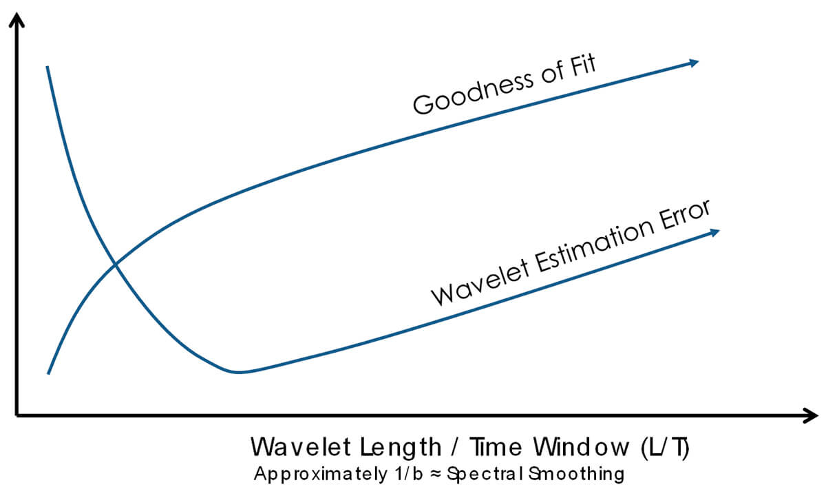
The longer the ratio L/T is, the better it can fit everything in the time window. But as the wavelet gets longer, the wavelet begins to also fit noise, and the wavelet estimation error goes up. At the opposite end of the axis, the goodness of fit is poor, as we are over-smoothing in the spectral domain. The idea is to find the optimum zone, where the error is low and the goodness of fit is high.

Phase determination: the good and the bad tie

Goodness of fit can be analyzed as a function of phase and time-shift (or time delay). An example of a good tie using high bandwidth data is shown in Figure 7.

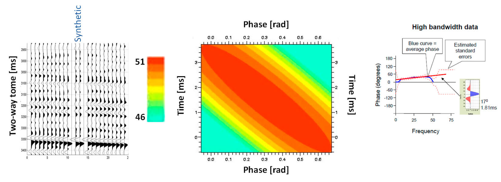
In Figure 7, we can see there is a trade-off between goodness of fit and phase, but in this example the phase spectrum is quite tightly constrained and uncertainty in the phase is about 10 degrees. We can conclude that this is a good tie.

Opposite to this example, Figure 8 shows a bad tie in a low-bandwidth dataset.

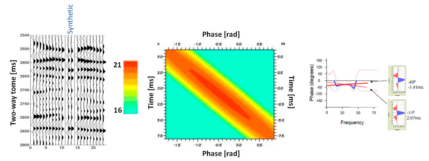
A similar trade-off as in Figure 7 is seen, but the phase spectrum is poorly constrained and the uncertainty in the phase is high. We can also see that qualitatively speaking, when comparing the synthetic trace with the seismic data just visually, the tie in Figure 8 looks acceptable, however, we showed that phase is poorly constrained and therefore this is a bad tie.

The fairway for good wavelet estimations

In practice, the seismic bandwidth, the wavelet length L, and the seismic time window T are related (Figure 9).

In Figure 9, the frequency bandwidth ‘B’ of the seismic data determines the optimum effective wavelet length ‘L’ required for a synthetic to match, which in turn limits the range of well synthetic time windows ‘T’ that can be used as input to wavelet estimation. This seismic bandwidth can be determined using a statistical wavelet estimation or by any standard spectral analysis software and checked against any filtering applied by the seismic processing sequence.

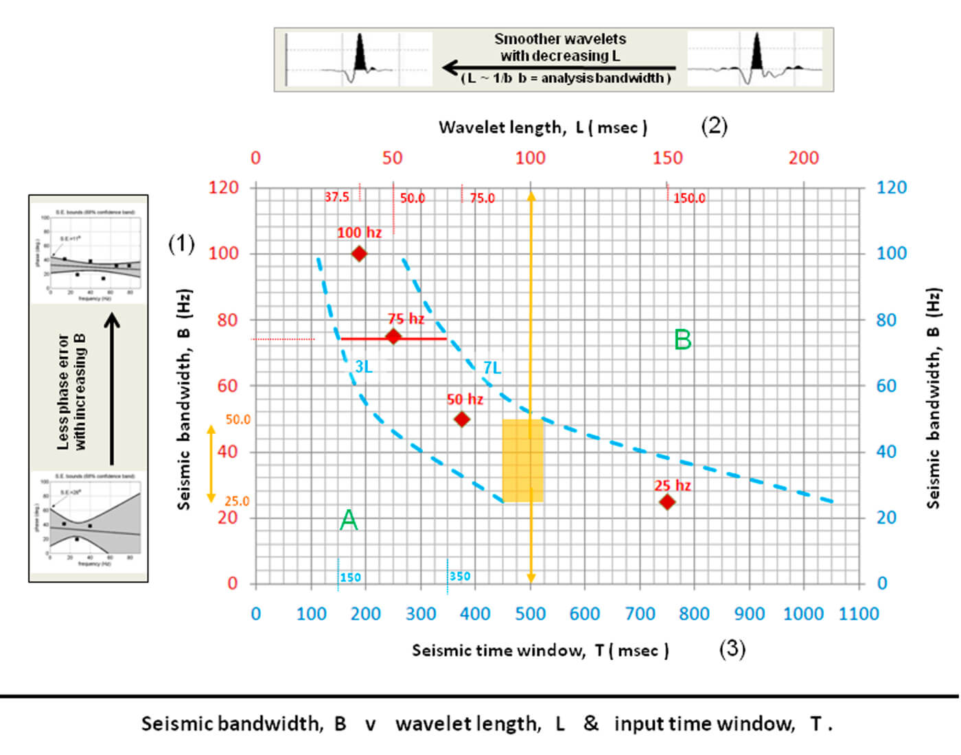
The graph shows frequency bandwidth versus optimum wavelet length (red X, Y axes, and red diamond points) and frequency bandwidth versus time window min. and max. (blue X, Y axes, and blue dashed lines).

The more bandwidth the seismic data has, the shorter the wavelet should be, and therefore, the shorter the input seismic data time windows recommended for best results. In Figure 9, the wavelet length axis numbers are 1/5^th of the time window axis numbers eg: L = 100 msec is also T = 500 msec. The range of recommended input time windows, for a wavelet of length L, is given by the two dashed lines, 3L & 7L, which together outline the “fairway” within which good wavelet estimations should be possible.

Given a seismic data frequency bandwidth B of 75 Hz (axis [1], side) (e.g.: bandpass filtered to be 5 - 80 Hz, 10 - 85 Hz , 20 - 95 Hz, etc.), we can see from the graph that the recommended optimum wavelet length L would be 50 msec (axis [2], top) and that this length corresponds to a time window T range of 150 – 350 msec (axis [3], bottom).

Reducing wavelet length, given a fixed seismic data frequency bandwidth, will create smoother wavelets from this wavelet estimation process. The more seismic frequencies that can be included in the input seismic trace, the better the phase estimation, as more points are available to define the wavelet’s phase line (see the cartoons beside the B, L, T plot in Figure 9).

Historically, most seismic data contained frequencies between 10 and 60 Hz near the surface reducing to 10 – 35 Hz or so in the deeper section. In other words, between seismic frequency bandwidths of 50 and 25 Hz. These bandwidths correspond to wavelet lengths around 100 msec and seismic input time windows around 500 msec, which is why they are often set as defaults in Roy White wavelet estimation (see orange annotation and rectangle in diagram). We use 124 msec for “well synthetic time window length/effective wavelet length” and 500 msec for “cross correlation range” defaults in RokDoc.

The green A indicates an area on the graph where distortion of the estimated wavelet is likely because the wavelet is too short for the seismic data’s restricted frequency bandwidth and B indicates an area where longer wavelets than necessary allow noise to be matched to the synthetic as well as signal.

Examples of workflows risking distortion (A) might be:

• Estimating a low frequency bandwidth far offset wavelet, reusing inappropriate near offset (i.e., higher-frequency bandwidth based) L and T parameters.
• When forced to use a well synthetic time window T that is “too short”, because the well’s sonic logs were recorded over a restricted time range.

Examples of workflows risking matching noise (B) might be:

• Using well synthetic time windows T that are long enough to allow matching of surface multiples as well as primary signal.

It is better to make wavelets too long than too short in most cases.

Well tie example

We have a dataset consisting of five wells and seismic angle stacks of the Norton oil and gas field located offshore Australia in the Carnarvon Basin. The five wells have a complete suite of logs as well as shear sonic logs. Gas is observed to the southwest of the field in well Norton 5, slightly gassy oil in well Norton 1, oil in wells Norton 3 and 4, and brine in Norton 2. The seismic data comprise four partial stacks that have angle ranges of 8-19 degrees on the nears, 19-30 degrees on the mids, 30-41 degrees on the fars, and 34-45 degrees on the ultra-fars. There is an overlap in the angle ranges of the fars and ultra fars stacks, meaning that we are sampling these angles twice. We reduced the weight of the fars and ultra-fars in the inversion to account for that.

The arbitrary line shown in Figure 10 connects the five well locations. The Jubilee sand is our main reservoir; it has a low gamma-ray signature and porosities in the mid 20’s percent. We can see a strong trough at the top of the Jubilee sand. The seabed peak indicates that we are dealing with SEG (North American) normal polarity where a peak corresponds to an increase in acoustic impedance. Another important amplitude anomaly is observed in the well Norton 1 (indicated by a black arrow in Figure 10). This anomaly represents hydrocarbon-bearing sand at this location. Aside of Jubilee and Ranger sands, the rest of the section is largely shale. There are seismic artifacts related to the presence of a seabed canyon located around the Norton 5 well. These artifacts include an amplitude washout in a vertical strip below it and multiples at the base of the section.

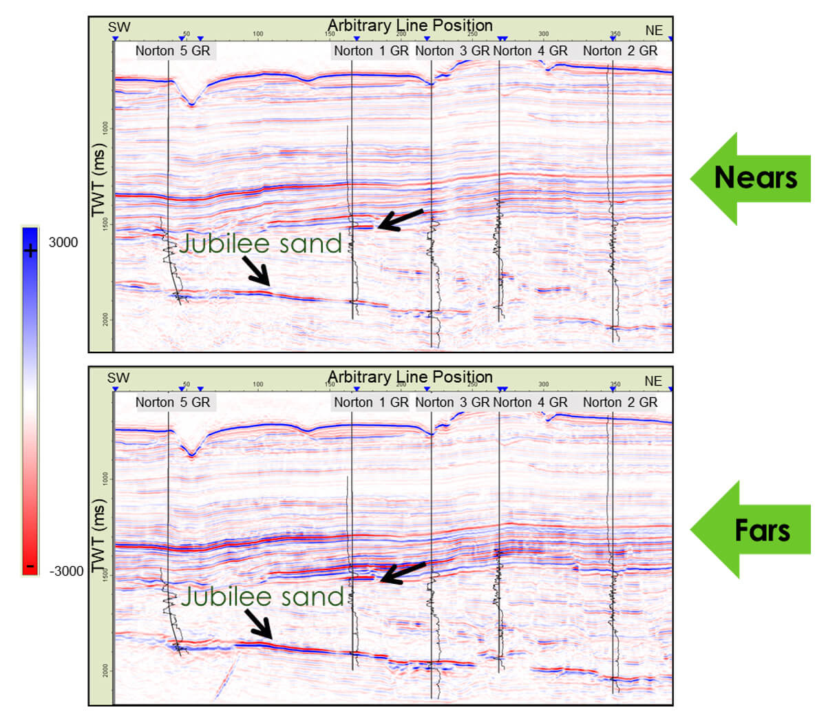
The Jubilee sand is mainly a Class II/III AVO seismic anomaly; overall, there is an amplitude brightening observed at the far stacks when we compared it to the near stack in the whole line (Figure 10). These AVO effects are present in the hydrocarbon-bearing sand but are also observed in the water leg. Fortunately, we have well data in the brine and hydrocarbon sands; therefore, we have known fluid properties that facilitate the calibration of the seismic response and reliable inversion results.

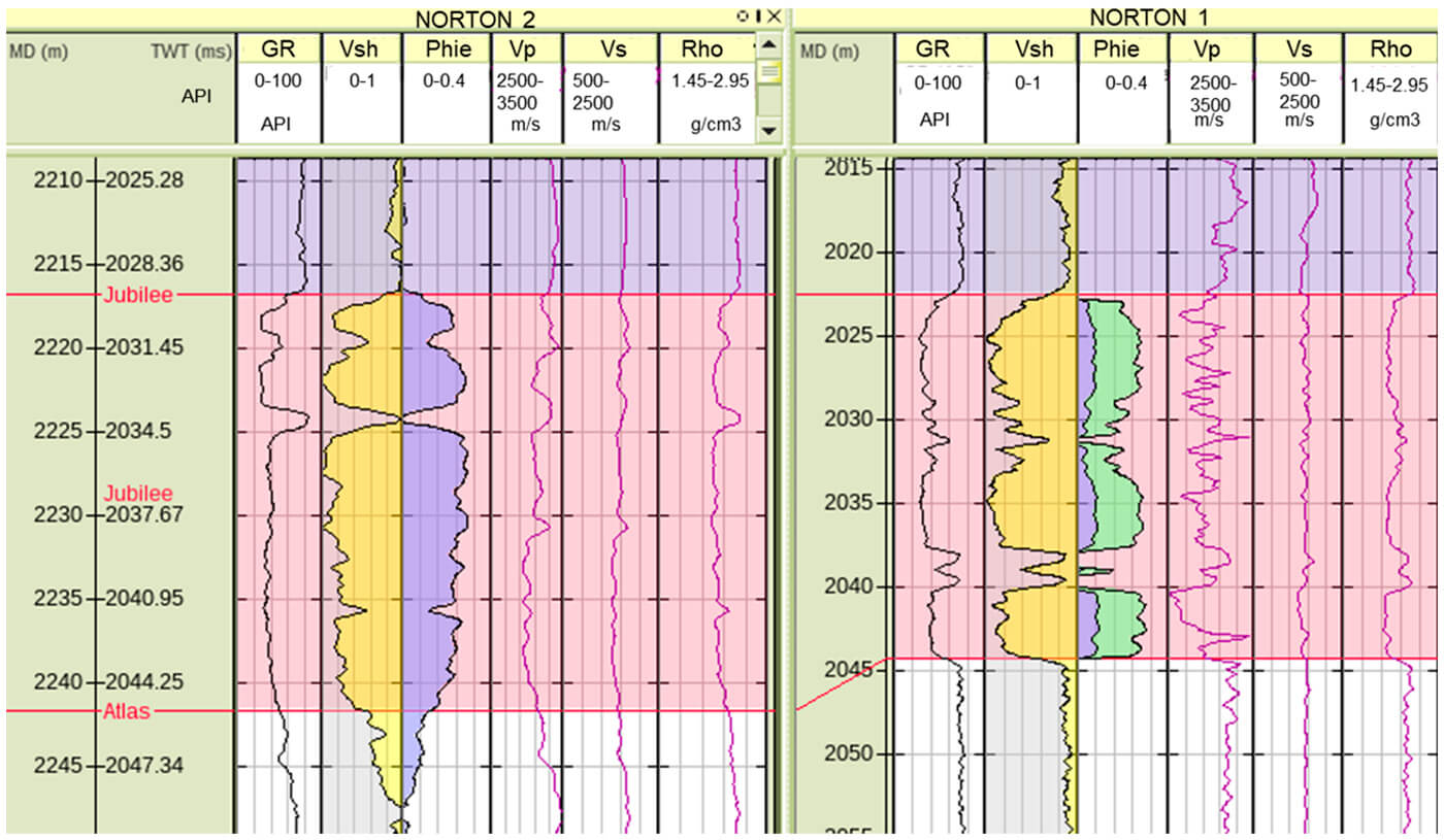
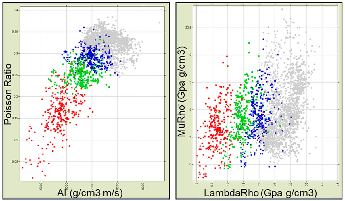
The Jubilee sand is our main zone of interest in wells Norton 1 and 2. It is highlighted in red in Figure 11. These wells are plotted side by side and were flattened at the Jubilee marker top. Norton 1 is oil saturated, and Norton 2 is brine saturated; you can see anomalous low p-wave velocity values in the well Norton 1. To better discriminate fluids and lithologies, we cross-plotted the data in the elastic property space (Figure 12). We can observe a clear separation between the different fluid cases: brine, oil, and gas are shown in blue, green, and red, respectively. Lithologies are also discriminated in these cross-plots, the sand separates from the surrounding shales, shown in grey. These results are encouraging because they indicate that the pre-stack inversion outputs: Vp, Vs, and Rho can be used for reservoir characterization of this field.

In this case study, we want to demonstrate the importance of a good well tie for optimal seismic inversion results. We focus specifically on the role of the wavelet and we inverted the seismic data by using two set of wavelets following our suggested methodology. We estimated wavelets at the five well locations for each partial stack, meaning that we estimated a total of 20 wavelets. Then, we average them to get a wavelet for the nears, the mids, the fars and the ultrafars, and this is what we called a set of wavelets. This process is only possible if there is consistency between the wavelets across the angle range, with only gradual variation in the form of a decrease in bandwidth and modest phase rotation from the near to far stacks. Otherwise, data conditioning is needed to have better results in the seismic inversion.

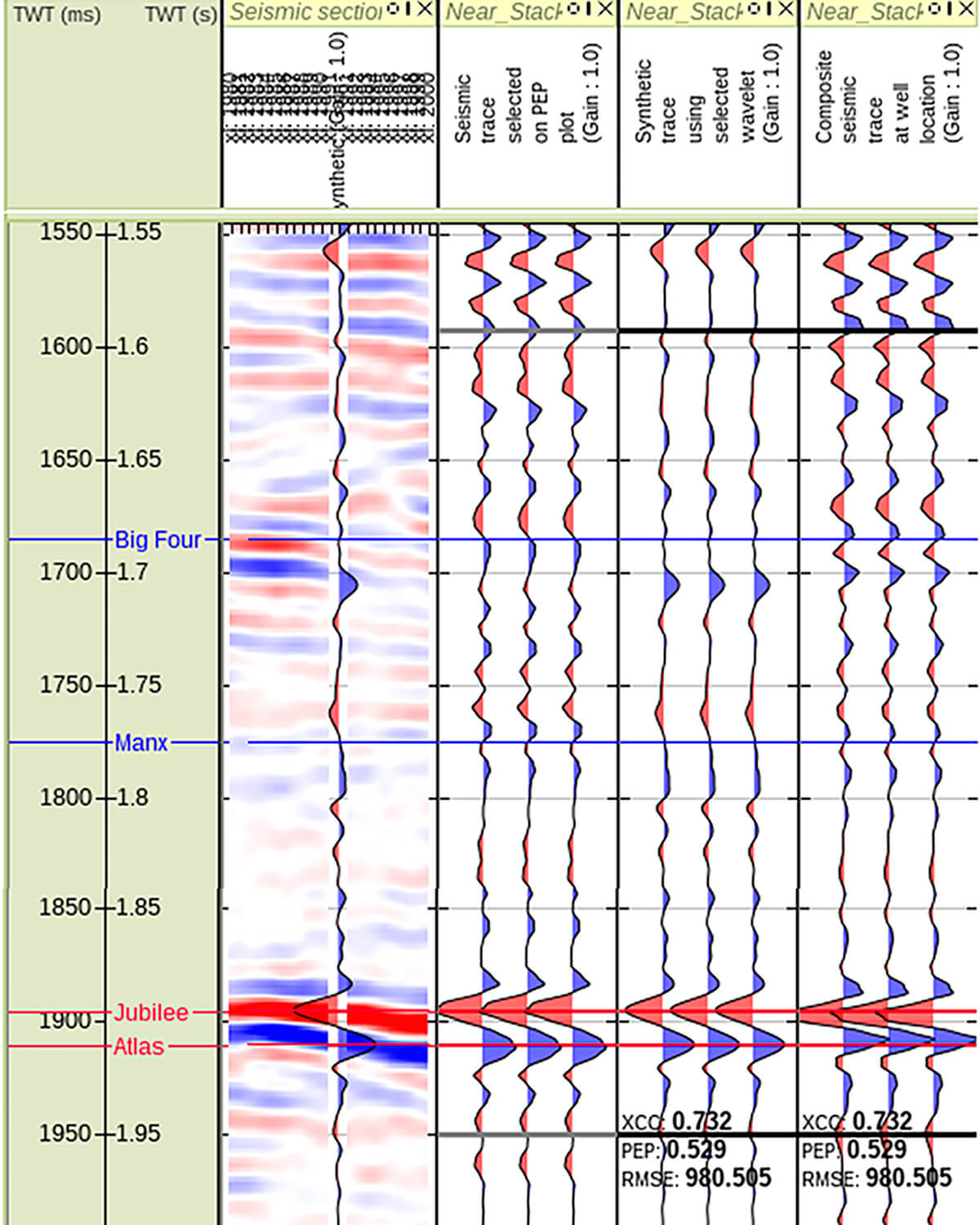
Figure 13 shows the well tie in the well Norton 1 for the near stack. There are four tracks, from left to right: the first one shows the seismic section with the synthetic trace at zero angle of incidence, the next track is the seismic trace selected at the best PEP location, then the synthetic trace using the estimated wavelet, and the last track is the composite seismic trace estimated at the well location. Visually, we can observe a good well tie, especially at the top of the target in the Jubilee sand. Above the target the section is noisier, but still we have a reasonable tie with a cross-correlation value of 73% in the window from 1590 to 1950 ms.

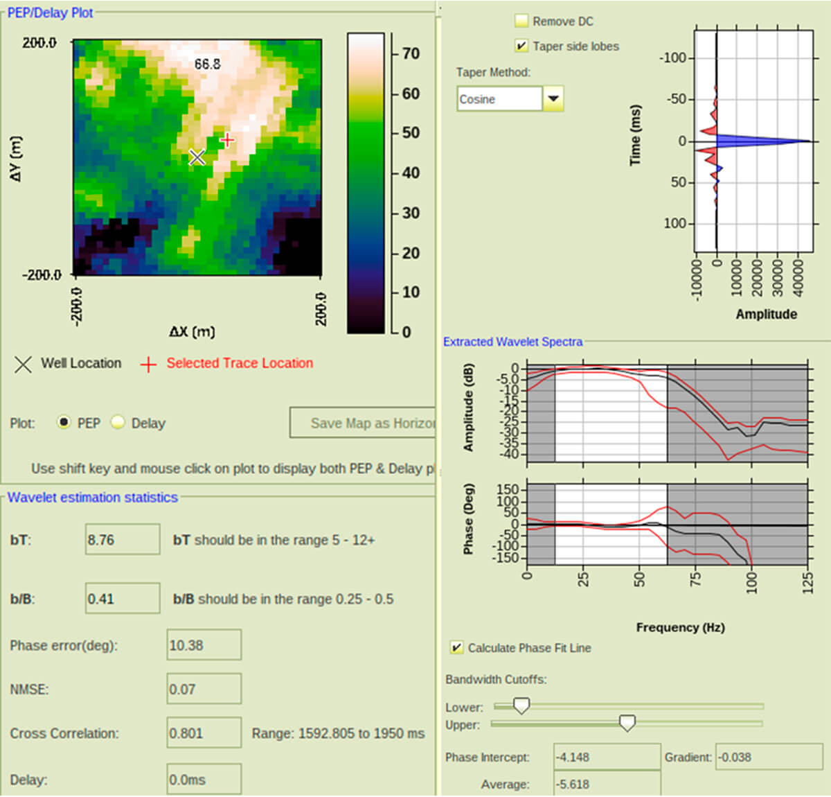
The quantitative analysis of our synthetic well tie for the near stack is shown in Figure 14. The proportion of energy predicted (PEP) over a 200 m square window around the well location is shown in Figure 14. Note that the best PEP values are observed around 50 m away from the well (identified with a red cross). Although high PEP values indicate a good synthetic tie, we also need to look at the delay. We selected the best well tie that satisfies both a high PEP value with near-zero delay and estimated the wavelet at this location. The NMSE value of our estimated wavelet is 0.07, which meets the criteria of a number below 0.2. The analysis bandwidth times the window length (bt) and the analysis bandwidth of the seismic (b/B) are inside the recommended values. For both parameters, low values indicate the wavelet is under smoothed and the wavelet length should be decreased and high values indicate the wavelet is over smoothed and the wavelet length should be increased. The average phase of the wavelet is -5 degrees and the phase average error is low at 10.38 degrees. We repeated this methodology for all the partial stacks and wells and averaged the wavelets per angle.

Looking good?: The effect of a qualitative well tie in seismic inversion

To evaluate quantitatively the effect of a qualitative well tie, e.g., tying a well based on how good it ‘looks’, we proceed to phase rotate all the average wavelets estimated using the Roy White methodology we used on our previous example -42 degrees.

Figure 15 shows that qualitatively speaking both wavelets (estimated and estimated rotated -42 degress) show a relatively similar ‘tie’ around the reservoir of interest (between the Jubilee and Atlas markers). However, when performing seismic inversion (in this case we calculated a quick Simultaneous Seismic Inversion), it shows two different results.

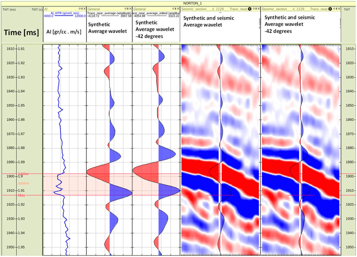
Figure 16 show the results of simultaneous seismic inversion using the estimated average wavelets per angle and when rotating them -42 degrees for compressional velocity (Vp) and Young’s modulus (E).

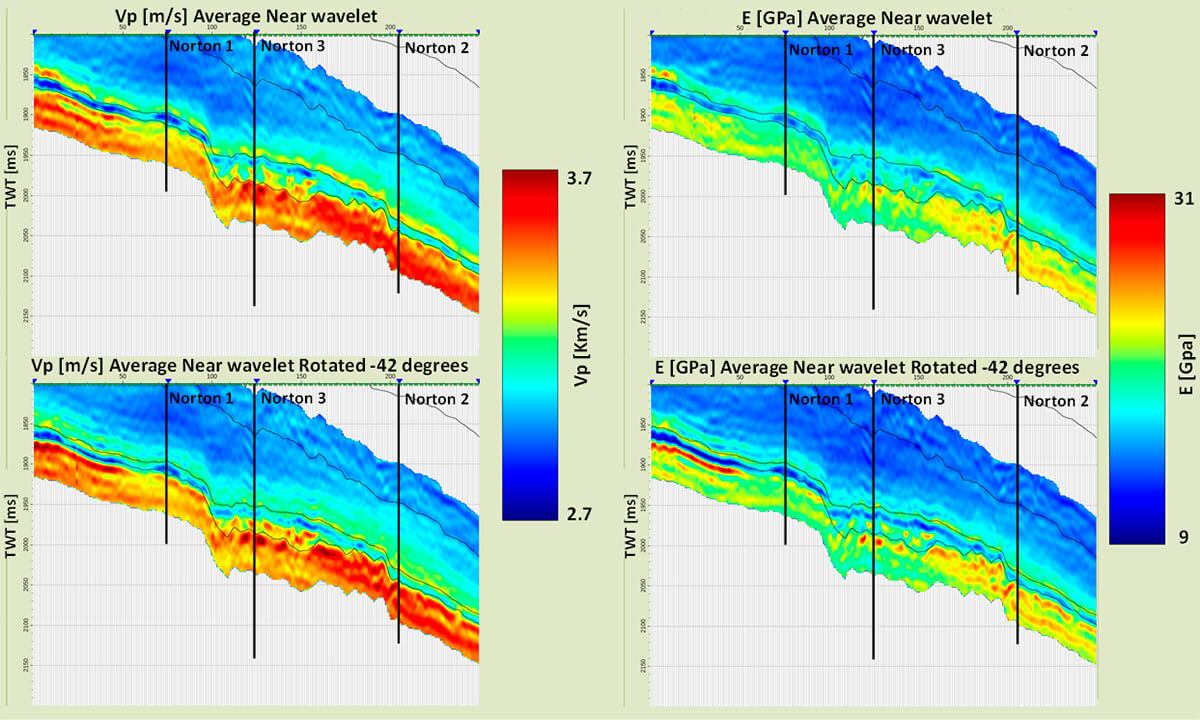
Even though we could see that the average wavelet rotated -42 degrees showed a ‘good’ match to the seismic stack at the reservoir level (Figure 15), it is clear now that after removing the effect of the wavelet through the seismic inversion process the elastic properties will be different from those estimated using the right wavelets. This effect is seen not only on the position in time of the maximum values but also the magnitude itself is different.

Because there was a phase rotation applied to the estimated wavelets, the values of elastic and geomechanical properties appear to be shifted in time (Figure 16). Relative differences from the Young’s modulus estimated from original and rotated wavelets can be seen in Figure 17.

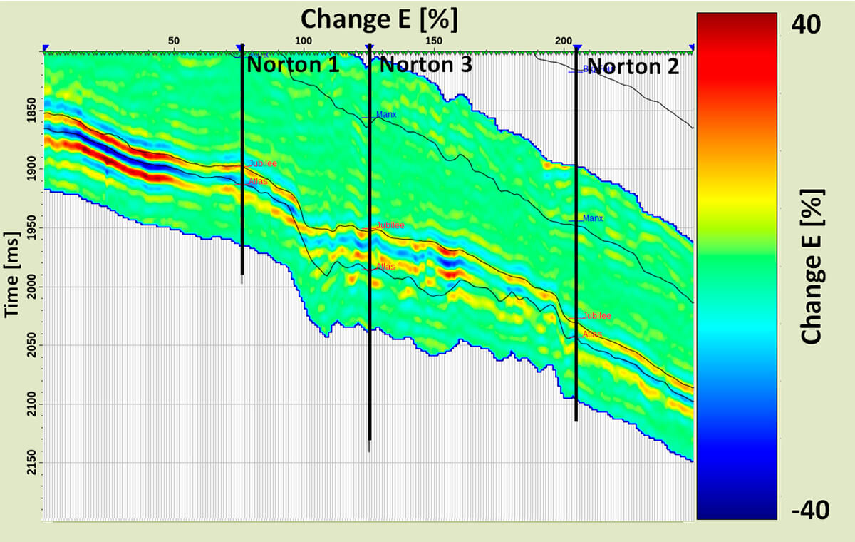
Changes in Young’s modulus values, are shown to be as high as ±40%. We know this is due to the fact that the properties appeared to be shifted when using the rotated wavelets, but it is important to mention, as we know, that position in time will affect the position in depth and therefore may affect drilling planning. Moreover, in this example, the extreme changes in E (+40% and -40%) seems to be linked with the pressence of gas (updip, to the left of Figure 17, is known to be gas). This fluid effect may increase even more the uncertainties of elastic properties calculated from seismic inversion when the wavelets are not the correct ones.

Conclusions

Well tie is a very important and often overlooked step in seismic interpretation and seismic inversion. The process of well tie involves the process of wavelet estimation, from which we obtain the different angle-dependent wavelets that are used in the seismic inversion process. Qualitative wavelet estimations can affect the estimated elastic parameters from seismic inversion in a negative way. Quantitative methods, on the other hand, can provide a way of measuring uncertainties of amplitude and phase of the wavelets. Concepts such as PEP and NSME provide additional information as a way of evaluating and demonstrating good wavelet estimates and the wavelet estimation parameters can be determined using the "fairway for good wavelet estimations” from Figure 9. Finally, it was shown that predictions of geomechanical properties could be significantly affected by the estimated phase.