VSP for the Interpreter/Processor for 2001 and Beyond: Part 1

Abstract

The use of the Vertical Seismic Profile (VSP) has expanded during the past 20 years into an economical and viable exploration and exploitation tool. Having started as an extension to the Check Shot survey, an interpreted VSP dataset is seen as a high-resolution subsurface image that is the intimate link between geology and geophysics - it supplies a ground truth to our surface seismic imaging.

In this paper, we shall review the status of the VSP method today in light of the progress of the last 20 years and of what lies ahead. The theme of interpretive processing will be key to the VSP method in our day-to-day exploration needs. We will review interpretive processing, the revolution in acquisition (both source and receivers), and the contribution of the method to the 3-D surface seismic world.

Introduction

A historical review of the VSP method can be found in Hardage (2000). The borehole seismic method has been historically thought of as the Check Shot survey. This survey consists of placing a receiver down the borehole at large depth intervals and sending acoustic energy down to the receiver from a surface source. The first break time of the initial arriving energy is picked and the time depth data is used to calculate seismic propagation velocities and, ultimately, interval velocities between the receivers’ depth levels. Knowing the interval velocities down the borehole, a sonic log can be calibrated to tie the seismic data using the Check Shot data. One does start to ask the question, “Is this not backwards, using VSP seismic data to correct a sonic log (synthetic seismogram) to tie surface seismic data? Why not just use the VSP data itself to tie the surface seismic two-way traveltime to depth?”

We will see this question in another form when we discuss tomography data (part 2). The Check Shot survey and the VSP can be viewed in the same light as the crosswell transmission and reflection tomography. One set (the Check Shot and transmission tomography) uses first break arrivals, while the VSP and reflection tomography use first break and later arriving reflection data to image the subsurface.

To work with the VSP data, we look at the down- and upgoing events. The events can be interpreted by noting an event’s traveltime change with changing receiver depth. As the downhole receivers (sondes) are lowered down the borehole, the downgoing events increase in traveltime from the surface source to the sonde. The traveltime of the upgoing events will decrease since the sonde is getting nearer to the reflector that created the upgoing event. Once the sonde is below the reflector of a particular upgoing event, then that upgoing event ceases to be recorded. This says that the first break downgoing event is the same as the upgoing event at the location of the reflector that created the upgoing event. The depth value of the recorded trace at this point is the depth of the reflector that is being imaged by the upgoing event. Figure 1 shows the concept of up- and downgoing events using a model and real data.

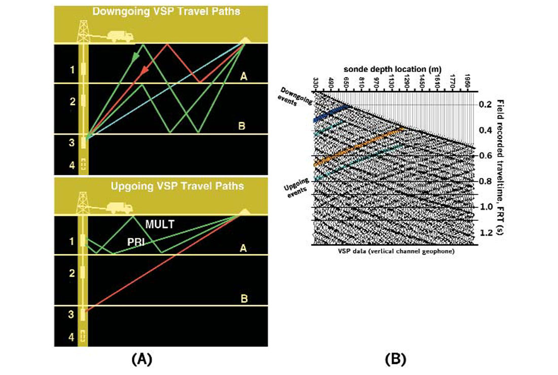
In Figure 1 (A), the only primary downgoing event is the direct arrival (or the old check shot raypath). This means that any downgoing event that trends parallel to the direct arrival is a multiple; the ray has reflected up and back down during its path to the sonde. The primary events will intersect the first break curve as is seen in part (B) of the Figure 1. The blue and the orange events are primary reflections. The upgoing multiple from a reflector cannot be recorded below the reflector. This can be seen by the light blue events that are multiples of the dark blue and orange events. The multiple events do not intersect the first break curve and they are not recorded beneath the reflector that created them.

To correct the upgoing event on a zero-offset VSP to two-way traveltime, we add a trace’s first break time to the trace as a bulk shift. We call this time frame +TT time. To separate the up- and downgoing events, we can apply velocity based filters, median filters and other filters that take advantage of the similar but opposite dip of the up- and downgoing events.

Interpretive Processing

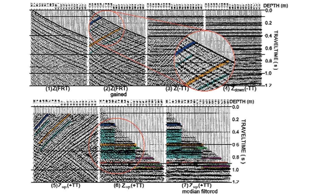
The VSP dataset is a small amount of data compared to surface seismic data. When we wavefield separate, gain or deconvolve the VSP data, bad choices of processing parameters can destroy data or create false data artifacts which could be mis-interpreted as geology. We have suggested a methodology called interpretive processing for the VSP user. The interpretive processing panels display the processing flow and enable the interpreter to examine everything that has been done to their data. More importantly, the panels allow the interpreter to fully examine the VSP data in the same manner as they quality control surface seismic data processing. An example of an interpretive processing panel for wavefield separation is shown in Figure 2.

An entire series of processing panels can be generated for (see Hinds at al., 1996):

• zero-offset VSP wavefield separation
• zero-offset VSP deconvolution
• zero-offset VSP corridor stacks (both deconvolved and nondeconvolved data)
• far-offset constant angle polarization
• far-offset time variant polarization
• far-offset VSPCDP/migration

For the far-offset processing, it is crucial that the interpreter examines the redistribution of the X, Y and Z data all the way out to the VSPCDP transform. The polarizations result from the triaxial nature of the sonde. The X, Y and Z geophones in the sonde in a far-offset VSP capture non-vertical incident wavefields. This means that the up- and downgoing P and SV waves are distributed onto all three axes.

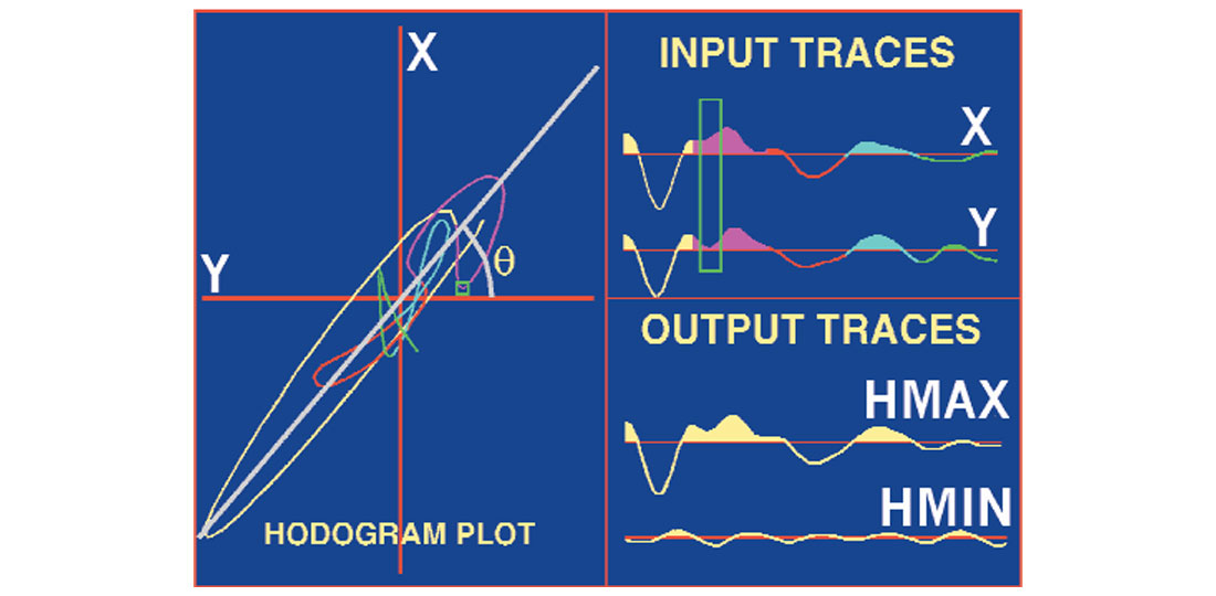
The first set of polarizations examined using interpretive processing pertains to the “rotating” the P and SV data of the two horizontal channels into the plane of the well and the source. This is done by analyzing a window of data around the first break. The data from the X and Y channels are plotted onto a hodogram diagram (see Fig. 3). The hodogram analysis outputs an azimuth angle that relates to the angle between the Y-axis and the plane of the source and well. The plotted data are colored coded to enable the interpreter to fully examine what portion of the windowed data is making what part of the hodogram figure.

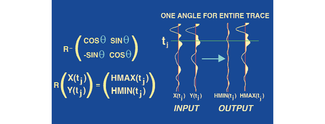
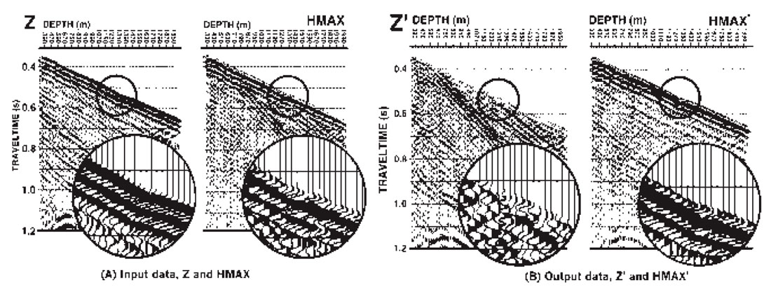
In Figure 4, we see the matrix formulation of the polarization process. The point to emphasize here is that we use one angle per pair of input traces. Now we look at the Z and HMAX data that lie in the plane of the source and the well. We want to separate the downgoing P wave onto a single panel and then isolate these events in order to (1) use the downgoing events for far-offset VSP deconvolution and (2) get a clearer picture of the upgoing events. We apply the hodogram analysis to the Z and HMAX data to output the Z’ and HMAX’ data. The input and output data are shown in Figure 5.

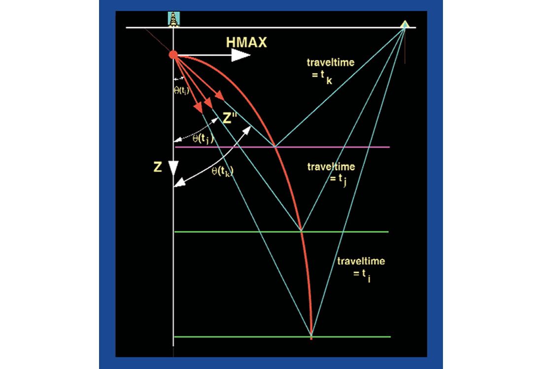
At this point, one might think that only upgoing P-wave events would be resident on the Z’ data panel. We can take the Z’ data panel, convert to two-way traveltime (+TT), migrate or VSPCDP transform from (depth, time) into (offset from well, time) and interpret. Well, we have one small issue; that is, as the reflections that arrive back up at the sonde originate from deeper and deeper reflectors, the angle of incidence and reflection at the reflector decrease. This can be seen in Figure 6. We have just talked about rotations (redistribution of two input data panels onto two new output data panels). These rotations used a single angle because we were performing a rotation into a plane or a rotation of the primary direct arrival (first break) towards a stationary source point. The reflections that arrive in the simplistic model in Figure 6 necessitate rotation angles that are time-variant. To find the angles, the reflection traveltimes and angles are calculated through ray tracing. The methodology is constrained using the interpreted upgoing VSP events in the data. The solution is an associated angle of emergence into the sonde for every trace time sample. The major reflectors are first used to evaluate a series of angles and traveltimes and then the remaining angles are interpolated.

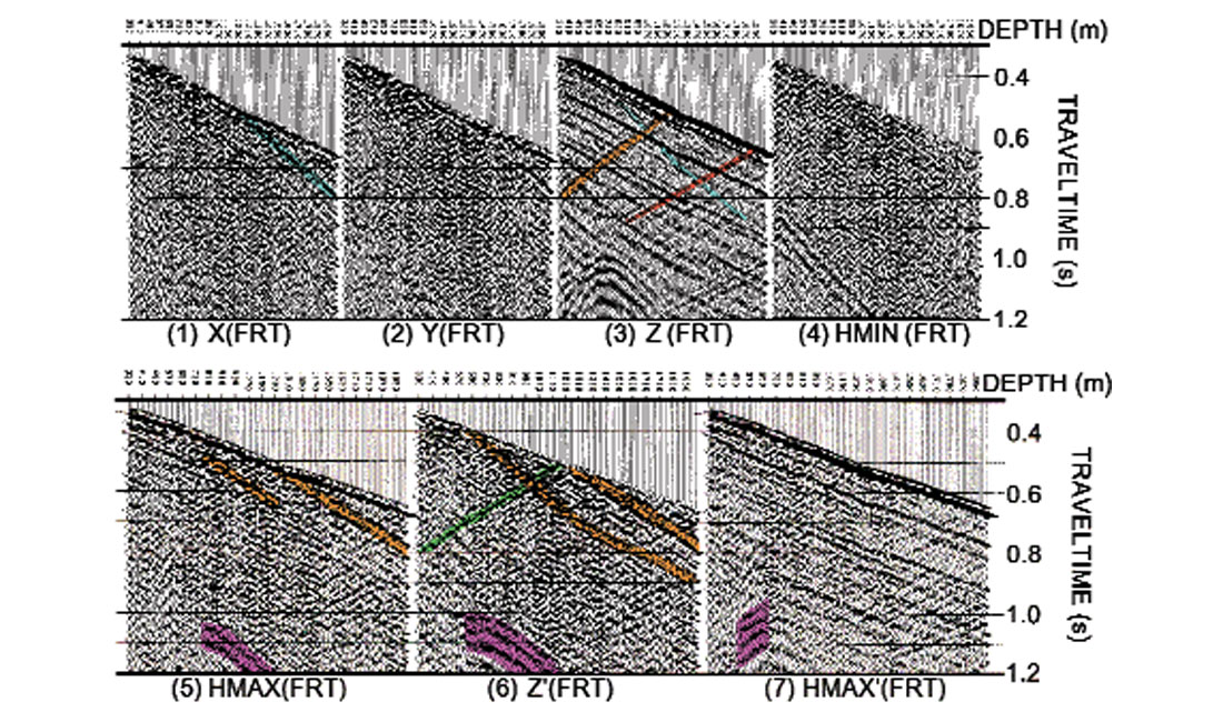
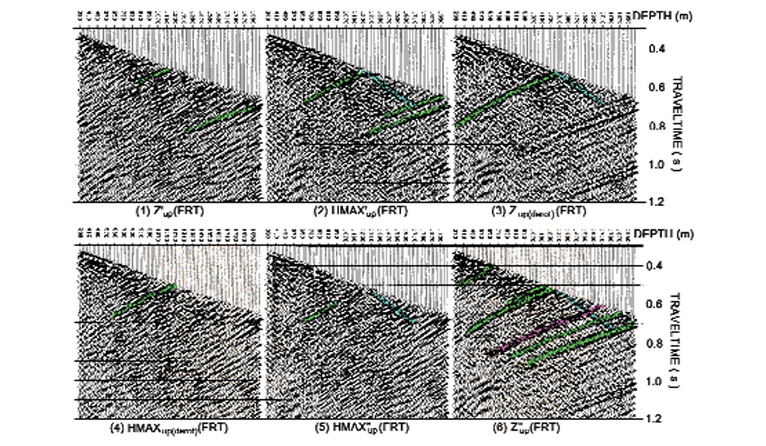
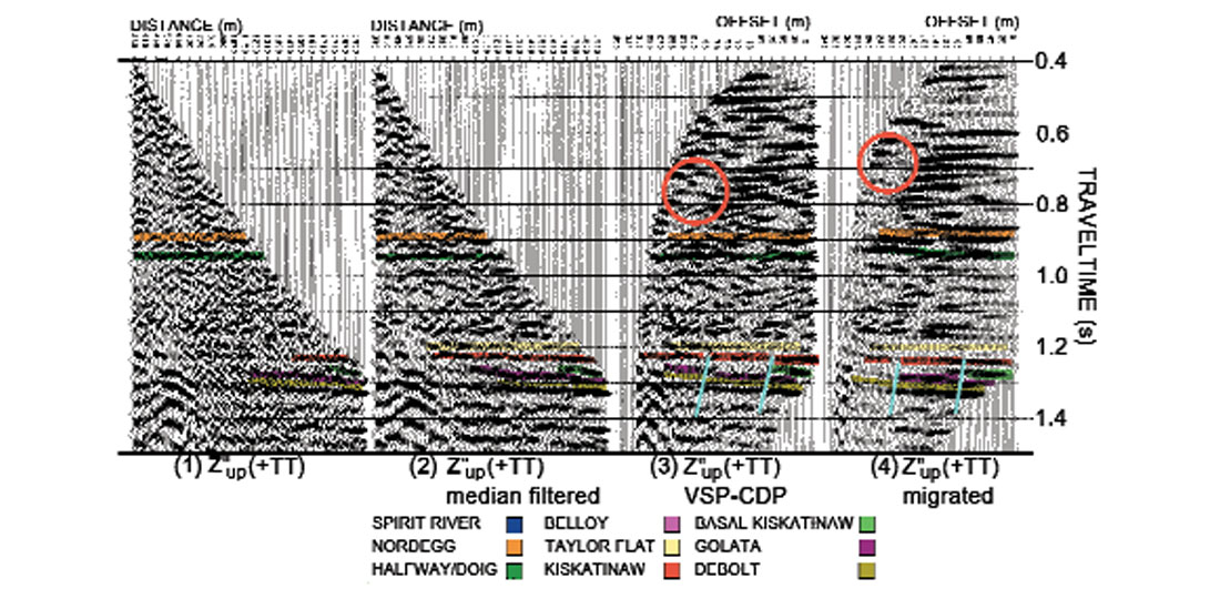
Two IPPs are constructed that show the series of data panels starting from the X, Y, and Z data and ending with the time-variantly polarized upgoing events (Figs. 7 and 8). The final time-variantly polarized data panels are termed Z” and HMAX” for convenience. The first IPP starts with the X, Y and Z data and ends with the rotated Z’ and HMAX’ data. The next IPP starts with the Z’upgoing and HMAX’upgoing and ends with the Z”upgoing and HMAX”upgoing. We assume that the far-offset survey upgoing events are isolated on the Z”upgoing data panel. For interpretative processing to work, one would thoroughly examine all of the data panels shown in Figures 7 and 8. In this dataset, there are a multitude of different types of data on each panel. We assume that the purple colored event is a diffraction from a nearby fault. The primary downgoing event changes on the X and Y data due to the rotation of the tool within the borehole in-between receiver station locations. Before decisions are made about the processing, these panels in practice should be fully interpreted!

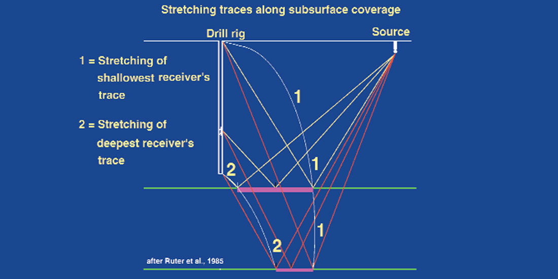
The data in this panel can be migrated or VSPCDP mapped. The VSPCDP mapping involves stretching the data trace over the reflection location curve. The transform came to light in the early 1980s (Wyatt and Wyatt, 1981; Dillon and Thomson, 1984; and Stewart, 1984). The coverage and two reflection location curves are shown in Figure 9. The VSPCDP and migrated Z”up data are shown in Figure 10. The VSPCDP’d data in panel 3 of Figure 10 shows two faults. The basal Kiskatinaw event in green exists at the well but truncates after the first fault is encountered. If one looks between 0.4 and 1.2 s on panel 3, linear noise trends are evident as washout zones amongst the “flattened” P-wave reflections. In interpretive processing, you would trace this noise pattern onto panel 2 and then onto the rotation IPPs. If that is done, there appear to be residual up- and downgoing shear events in the data. One can then redesign the processing sequence to counter the noise that is interfering with the VSPCDP mapped P-wave events.

The VSPCDP mapping was done on the example dataset using curved ray tracing. Another way to perform the mapping is to use an iterative approach to the mapping as discussed in Hardage (2000) and introduced in Chen and Peron (1998). One would alter the input velocities and layer definitions until the modeled VSP data matched the real VSP data. This would involve using geological data interacting with surface seismic data to give a geologically realizable input model. The integration of all available datasets assumes that the processing has been done the best it can be done.

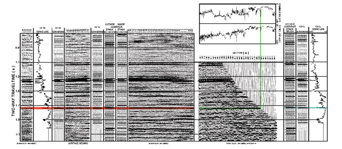
The VSP data can be presented with the seismic data by splicing in the VSPCDP data into the seismic section or the VSP data can be used to tie into an exploration picture using the integrated interpretive display (IID). Such a display is shown in Figure 11. To utilize this display, one would find a sonic or gamma anomaly that ties to a geological top. The VSP display and the log displays are tied by a common depth axis. A line is drawn from the log feature down to the first break on the VSP data in two-way traveltime. The polarity of the event could be checked using the sonic and density logs (does the acoustic impedance increase of decrease across the geological interface). The interpretation is continued onto the surface seismic using corridor stacks. All of the VSP data has been processed bearing interpretation in mind.

Why bring this into a paper on current and new directions in VSP? VSP data is typically seen as log data. VSP data are presented in log-type displays and are not truly integrated into the exploration dataset as seismic data. When we do surface seismic data processing, we use numerous check panels to verify each step of the processing. Interpretive processing is that answer for the VSP data. However, because the VSP data is intimately linked to the geology, you can track the events from the start to the end of the processing.

The IID type display can be modified to include P-SV converted event VSP data. Converted wave VSP data are extremely useful in P-P and converted wave 3-D surface seismic exploration (Stewart and Gaiser, SEG course). One can predict that converted wave VSP subsurface images will become more routine - why ? ... because we record P and any SV converted wave data on our triaxial geophones anyway.

Acquisition

In surface seismic, one common idea 15-20 years ago was, “I don’t care how you record the data in the field, processing will fix it.” This may have been said due to the redundancy of data that is brought in from surface seismic recording. Conversely, the type of tools that one uses for geophysical studies is all-important. With the VSP data, we have use of the borehole for a short while and then normally do not have further access. So, recording the data the best that we can using the optimum sources, receivers, sonde locking arm and borehole conditions will help ensure that we bring home good data to work with. What has changed over the last 15-20 years and what’s ahead? Lots!

The two most important developments have been:

1. getting better geophone coupling to the formation
2. ensuring that tool resonance is not interfering with the recorded signal
3. making use of multiple sondes

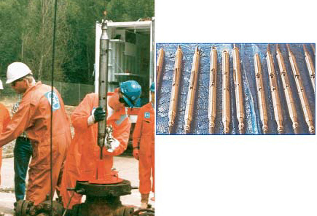
The early sondes were built to withstand the borehole environment (temperature and fluid). The geophone arrangement was a single vertical phone or three in a series. The number of vertical phones in series was limited by the seven-conductor wireline that was used on the logging trucks. The data came up the borehole through analog transmission. The tools were up to 3 m in height, had a locking arm that was screw driven (poor locking force) and weighed about 50-70 kg. An example of such a tool is shown in Figure 12. The weight of the tool was a factor in the geophone coupling to the formation (side of the borehole). When the use of two orthogonal horizontal geophones was considered in the older tools, the question of equal coupling to the formation of the X, Y and Z geophone became an issue.

The frequency and amplitude characteristics of the three phones should be as close as possible, if not equal. The older heavy tools required a substantial horizontal locking force to attempt to satisfy this requirement. Eventually, a hydraulically assisted mechanical locking arm came to the market; however, the answer lay in decreasing the size of the sonde itself in addition to having a strong locking arm force.

There are two methods in which satisfy these requirements. The first is to have a small movable part of the tool that houses the geophone package and to deploy that package out of the tool and force it towards the wall of the borehole (or casing). The second method is to decrease the size of the tool to a point where the locking force of the tool exceeds the weight of the tool by 5-10 times the tool weight.

The CSI tool designed by Schlumberger has a deployable geophone package. The deployed package contains an X, Y, and Z gimbaled geophone and a shaker device to measure the coupling to the borehole. The signal is digitized downhole at the receiver and sent uphole. The tool configuration can put up to 7 sondes into the borehole at any one time, and that shortens the data collection time.

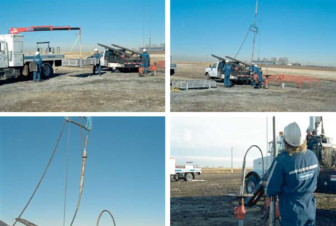
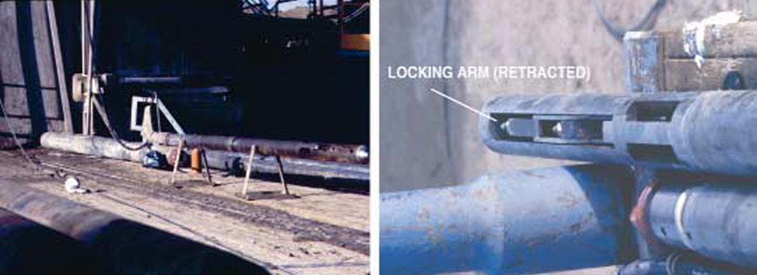
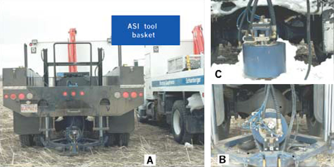
The 5-sonde ASI tool was designed by Schlumberger to be run inside of casing. The sonde is small and lightweight. Its locking mechanism is not accomplished using a locking arm. It uses a magnetic clamping device. As shown in Figure 13, the VSP acquisition contractor can arrive at the well site after the work-over rig has deployed and cemented in casing (before perforating the hydrocarbon bearing geological unit and completing the well) and run the VSP survey. Many of the wells in western Canada that set casing and run a VSP are shallow wells in Southern Alberta. For shallow wells, the ASI tool can be used and specially designed mini- Vibroseis units can be deployed as the energy source. Since the sonde is triaxial, the “mini-Vibs “ have been designed to project both P- and Shear waves. This is done by adjusting the articulating mass to be either horizontal or vertical (see Figure 14).

In the older tools, the frequency range of the tool resonance overlapped with the seismic bandwidth. By decreasing the size of the tool and increasing the locking arm strength, current tools can avoid the resonance problem and record more usable signal. One such tool is the SST-500 used by CGG (Gehant et al., 1995). A picture of the tool and its deployment are shown in Figure 15. In the paper by Gehant et al., they show data collected by a conventional tool (1995) and the SST-500. The new tool is less responsive to tube wave noise and more responsive to signal (due to the increased locking arm strength). The tool resonance of the 811 mm length tool was over 500 Htz on the vertical and axial (horizontal geophone motion along the locking arm direction) geophone and 400 Htz for the transverse horizontal geophone.

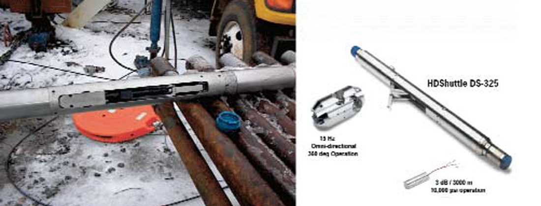
The next issue was the number of sondes that could be deployed at once down the borehole. During an SEG lecture, Rob Stewart stated that, “the perfect VSP configuration is where all of the geophone (sonde) locations are covered all at once and we shoot the surface source only once”. This can be coupled with the economic need to finish the survey with good data and in a timely manner; faster means less expensive. A number of tools are just coming onto the market that enable 20+ levels to be deployed at once. Geospace has developed a tool that has run 23 levels in Western Canada. The data transmission problem has been solved using fiber optics. A data collection shuttle is located in-between four sondes for analog to digital conversion. The digital data is then sent up to the beginning of the groups of sondes and linked to a fiber optic interface. The data then proceeds up to the surface using fiber optics in 24-bit mode. The tool also uses the Omni-phone. The Omni-phone is more sensitive to signal as the phone tilts than are the conventional geophones. A fourth receiver can be the addition of a hydrophone within the sonde. A photo of one of the Geospace sondes in the field and from a brochure is shown in Figure 16.

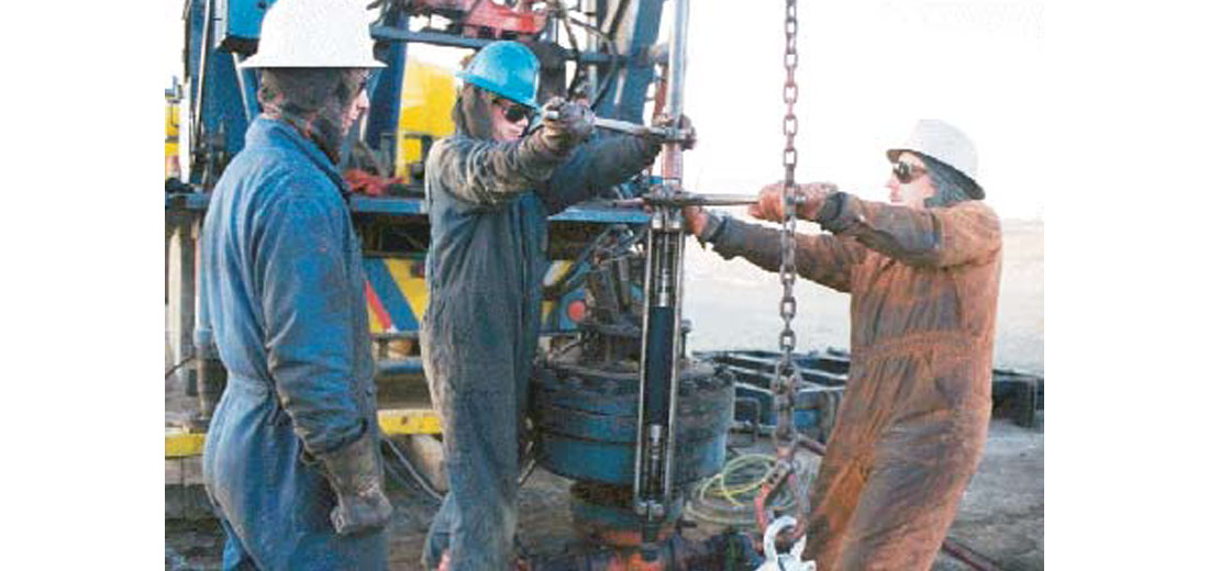
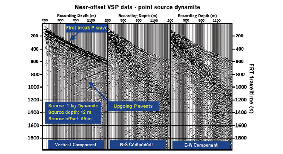
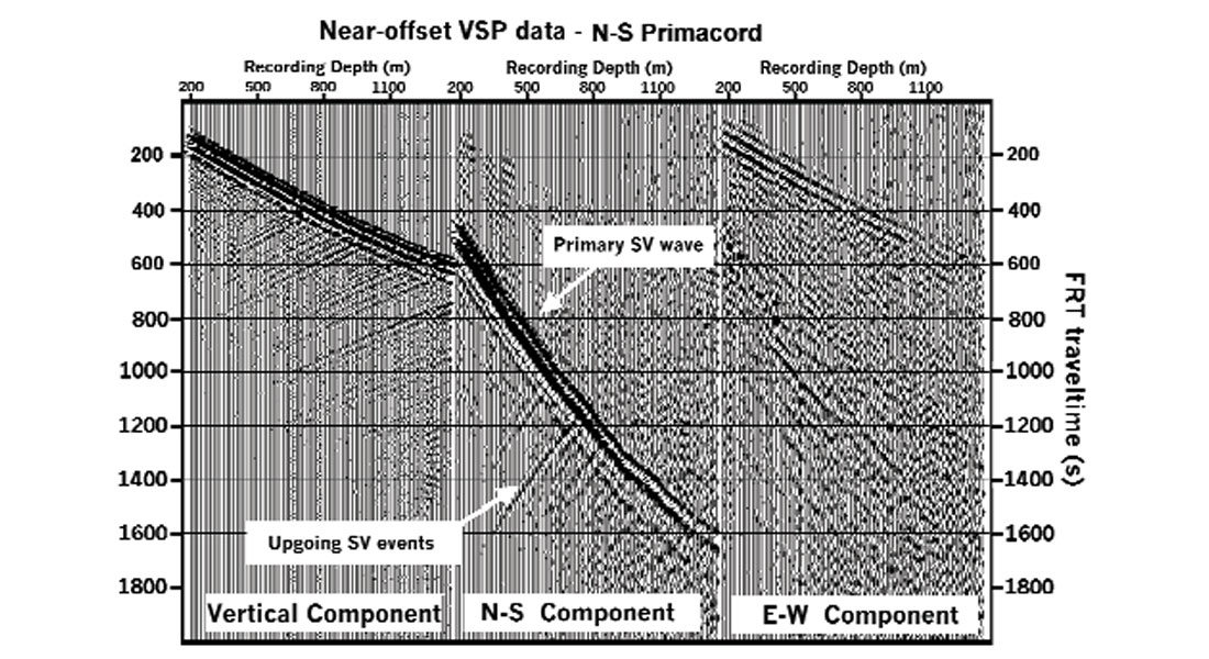
Another notable tool is the Paulsson Geophysical Inc. (Paulsson et al. 2001) 80 level tool. Yes, I did say 80 levels. The tool is constructed on-site by placing receivers within coil tubing. The tool deployment time depends on the construction of the 80 levels into the coil tubing. Each receiver package is triaxial and the data is of good quality. An example of the field deployment is shown in Figure 17. In this figure, the VSP crew is constructing the “continuous” tool within the coil tubing. VSP data obtained using a surface charge (point source) and line source are shown in Figures 18 and 19, respectively.

Overall, the tools have progressed a great distance from the heavy, long sondes of the 70s and 80s. Fiber optic cables (meaning analog to digital to optical) may eventually replace the analog to digital transfer of data to the surface. The stage is set to truly make the running of VSP surveys more economical.

3-D VSP surveys

The 3-D VSP started out as a poor cousin to the 3-D surface seismic survey. The VSP crew would set up 1-5 receiver levels in the borehole and the 3-D surface seismic crew would acquire data quite oblivious to the presence of the 3-D VSP survey using the surface seismic sources as VSP source points. Due to the small amount of VSP sonde locations that could be recorded in a single shot, the VSP crew either moved the VSP array up and down the borehole in order to broaden the vertical coverage of the VSP array or resigned themselves to processing in the common VSP receiver domain.

As highlighted in the previous sections, the number of VSP sondes in the VSP array is increasing. More of the borehole can be covered by the array than before. In a 1000 m borehole, a 30 sonde array with a 25 m receiver depth interval can cover can cover 725 m. There are several keys to the success of the 3-D VSP. Some are:

1. design the 3-D VSP field acquisition around the imaging of the zone of interest in accordance to the VSP geometry and not exclusively for the surface seismic geometry. The analysis of the modeling may suggest that infill shots be used in the area in addition to the normal surface seismic source lines;
2. recognize that the VSP is a seismic survey and not a logging run. This means that team cooperation between the surface seismic planners and the VSP survey planners is a must;
3. send a qualified VSP observer out to the VSP site. The observer should have joint-authority over the 3-D and VSP survey. (I recommend the geophysicist who is responsible for the exploration play);
4. participate in the field operations. Be on site before any surveys start (VSP or surface seismic) to quality control the placement and ground conditions of the VSP sources;
5. consider acquiring walkaway (for AVO and anisotropic studies) or any other source geometry VSP before the 3-D surface seismic survey begins; and
6. the processor and interpreter of the exploration project must act as a team if not being the same person.

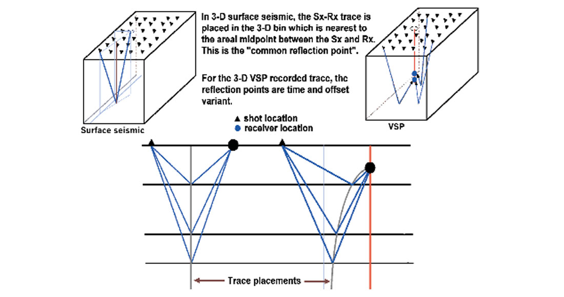
How does the reflection geometry of the 3-D VSP differ from that of 3-D surface seismic? The reflection point geometry for both surveys can be seen in Figure 20. The surface seismic geometry turns out to be the familiar common midpoint or “depth” point. The reflection point for the VSP depends on the location of the source point and the receiver location in the observation well. Figure 20 shows a 3-layer model and the reflection geometry for the VSP and surface seismic surveys. As expected for flat layers, the surface seismic survey geometry is the CMP. On the other hand, the reflection point geometry for the VSP is the VSPCDP curve of reflection points. For the VSP survey, the reflection points are time and space variant.

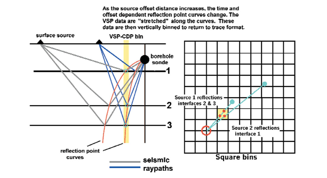
How do we do 3-D binning in the 3-D VSP survey? In Figure 21, a three-layer model is shown along with two inline seismic sources. In the yellow colored vertical bin, the furthest away source images layer 1 in the bin zone. The nearer source images both layer 2 and 3. In the bin plan map, 3 reflection points are in the bin. The key is that the reflections at layers 1 to 3 arrive at different traveltimes and corresponding modeled depths. One can conceptually envision the data trace from the far offset source being stretched over the VSPCDP curve and the data from the nearer offset trace being stretched along its reflection path. The data within the bin are then vertically re-binned in a similar manner to that of the far-offset single offset VSPCDP mapping. If the input velocity model is incorrect, then the reflections will be placed in other VSPCDP loci and may not locate in the correct vertical bins.

We have one more complication to discuss. What happens when we record and process the 3-D VSP data for P-P and P-SV reflections? Following Stewart (1991), the P-SV and P-P reflections from an interface recorded in a VSP survey are shown in Figure 22.

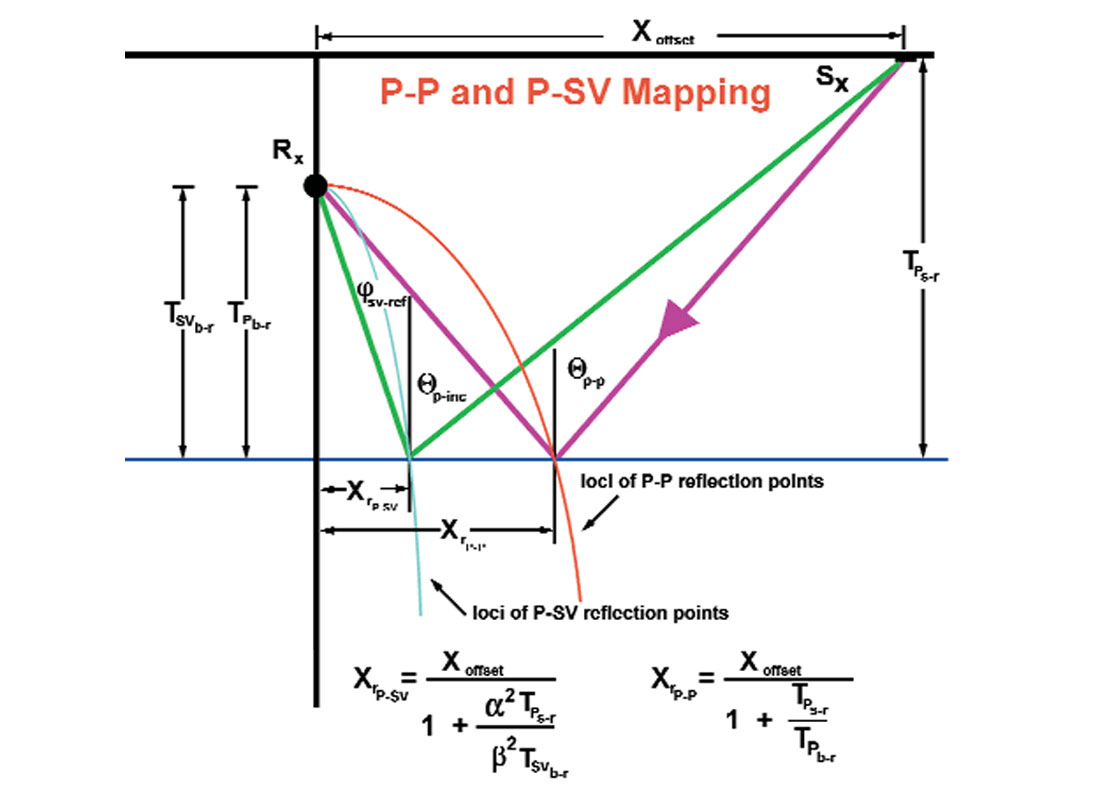
The traveltime equations follow Stewart (1991). The data trace would be stretched in two separate plots, one for the P-P reflections and one for the P-SV converted wave reflections. In pseudo two-way traveltime, the reflector would be located later in reflection time on the P-SV plot. In a depth plot, the reflector would be placed at the correct depth level; however, the reflection point for the P-SV reflection would be nearer the borehole than would be the P-P reflection point.

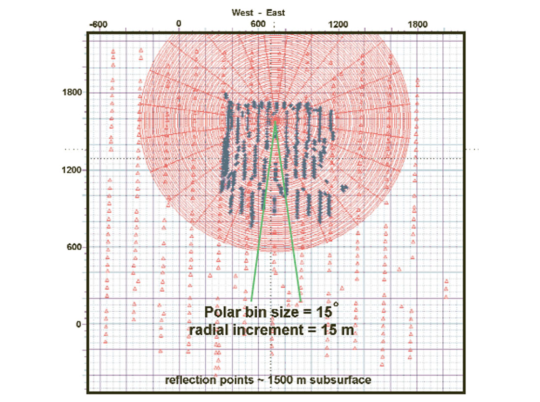
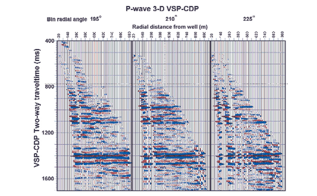
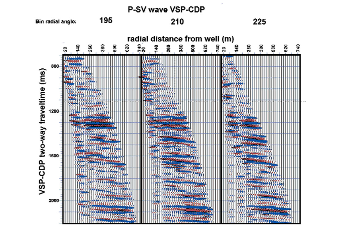
The binning can be rectangular or polar. The polar bins consist of radial lines projecting outward from the well and circles around the well at prescribed radial increments from the well. An example of the radial bins can be seen in Figure 23. VSPCDP mapped data representing 3 different radial directions for P-P and P-SV events are shown in Figures 24 and 25, respectively. The well is located on the left most trace of each of the three plots within Figures 24 and 25.

One of the most important pre-survey tasks is modeling. When we are dealing with the 3-D surface seismic survey, we model quantities like the surface seismic fold, coverage, decline of the coverage on the edges of the survey in very rectangular geometries (in-line and cross-line) and in the realm of common mid-points. We have just seen in Figures 20-22 that reflection geometry for a single source offset VSP survey is time and space variant and not the simple midpoint. When we have many sources at various azimuths around the well, the understanding of the subsurface fold becomes even more complicated. We can do 3-D VSP design modeling which looks at coverage along a reflector, the sonde locations that will optimize that coverage, and where the subsurface reflection points lie on a fold map. We can then add in source point location to build up fold where needed.

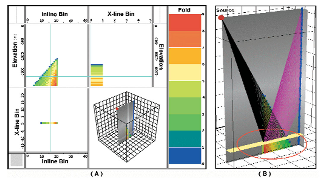
We should bear in mind that a basic subset of reflection points is provided to us through the normal rectangular 3-D surface seismic shot and receiver pattern. Example results from a modeling package can be seen in Figure 26. What can be noted in the increase in fold along the imaged reflector (in yellow) with increasing offset from the well. If the imaged reflector was raised to a shallower depth, the fold would decrease for a given bin location. Generally, the fold of the VSPCDP mapped data increases with increasing traveltime and offset from the well.

For the future, our attention will turn to cooperative modeling of the joint 3-D surface seismic and VSP surveys. The 3-D VSP survey will be a partner in exploration effort with the 3-D surface seismic survey. The interpreters and processors will quality control the VSP data as rigorously as they do the surface seismic and interpretive processing will be in both disciplines. The availability of multi-sonde tools will make the data collection more thorough and the economics of running 3-D VSPs more favorable.

Discussion

In this paper, we have reviewed interpretive processing, developments in VSP acquisition and 3-D VSP surveys. Interpretive processing will integrate into all aspects of VSP and its cousin, Crosswell Reflection Tomography. The world of VSP is moving ahead due to the advent of multi-sonde tools that will go a long way in making the survey more economical. The converted wave VSP interpretation should become a partner in the subsurface exploration. The ability to record and use the converted waves have been in the VSP survey for quite a while due to the triaxial geophone sondes. The link to the surface seismic 3-D world will be further enabled through integrated processing of both datasets. Through experience and opportunity, the asset teams in exploration companies will be able to fully utilize the VSP data for exploration and exploitation.

The message of the importance of field observation and quality control cannot be expressed more. VSP data is valuable in part due to the need for a wellbore and that wellbore is usually unavailable following the survey is completed. In the second paper of this series, we will examine AVO, 4-D VSP, Q, Anisotropy and the world of Crosswell reflection and transmission tomography.

Acknowledgements

We would like to thank Pancanadian Petroleum Ltd., and Computalog Ltd. for allowing us to publish this paper. We would also like to recognize and thank Paulsson Gephysical Inc., Schlumberger of Canada, Baker-Atlas (Baker Hughes Canada), CGG Canada Services Ltd., GEDCO/SIS and Oyo Geospace Corp., for their technical assistance and photos.